
8 TikTok Trends That Will Shape DIY and Home Decor in 2023

Scott predicts that limewash will be the portray approach to check out for in 2023. “We’ll see distinctive programs of limewash these kinds of as the cloud strategy to produce the glance of old worn walls,” he states. “Layering limewash in different means can give you the appear of 200-12 months-outdated walls—in just a few of days.”

5. Checkered styles

TikTok articles

This material can also be considered on the web site it originates from.

Proving that straightforward designs can have a large influence, check out print is possessing a moment—and that instant will continue into 2023. Lisa Buhler, the founder of the fashion line Lisa Claims Gah, thinks that people are drawn to checker print because it’s all about pleasure. She describes it as a “feel-very good print” that’s symmetrical but pleasurable. Haustile will take it a phase even further with a warped check out tile that seems to be like something out of an M.C. Escher illustration.

Interior designer and Do it yourself skilled Emily Shaw, regarded between her TikTok followers as @emilyrayna, is a proponent of this pattern. When working on her “finding-completely ready room,” she opted for a golden-rod-and-white checker print—with a budget-welcoming twist. “Checker print has been trending all in excess of TikTok in a variety of techniques, so I needed to come across a way to make the pattern functional,” she suggests.

Shaw ordered a picket box from Michaels and painted it the identical shade as the golden checkers. Then, she hooked up it to the wall, developing some dimension and a intelligent ring storage nook. “Emily, this is genius,” commented a TikTok follower. Agreed.

6. Combining multiple style themes

TikTok articles

This content material can also be seen on the web site it originates from.

According to the National Kitchen area & Bathtub Association (NKBA) 2023 Design Tendencies report, a single of the new tendencies this yr is combining various design themes to produce a one of a kind model. For example, natural and organic meets present day, or farmhouse satisfies modern.

Boston-based mostly Diy qualified Julie Sousa of @the_avantgarde embraced this fashion-blend trend in a new apartment redesign with her assistant Gigi Rodriguez. Sousa says that the most important type they have been following was contemporary, so they selected accordingly for the greater pieces—the couch, the chair, the espresso table, the ground lamps, and the mirrors. As Sousa clarifies even further, “The eclectic components occur from lesser parts like the wall art, the gold frames, and the usage of daring shades in the room.” Taken collectively, the complimentary kinds make the space sense up-to-date and personalized.

7. Generate spa-like bathrooms

TikTok written content

This material can also be viewed on the web page it originates from.

Because the commence of the pandemic, the collective tension has risen and is nevertheless to be abated. It helps make sense that persons have been impressed to develop calming, resort-like atmospheres in their own residences, in particular if they are still not traveling as much as they utilised to. NKBA found that spa-like bogs that “enhance property owner experiences” are just one of the major tendencies for 2023.

With its picket panels, calming lights, and lush plant wall, Sousa’s guest rest room revamp went viral on TikTok, garnering above 2.1 million sights. “I really desired it to truly feel spa-like, a position I could go to at the finish of a long day and zen out with a tub,” she states. Simply because the rest room was windowless, Sousa felt that greenery was the ideal way to distinction the moodiness of the black ceiling, not to mention, distract from the deficiency of home windows. “We usually affiliate greenery with a sense of freshness, especially in mix with drinking water and what superior space in the home than in a bathroom to build that notion of freshness and cleanliness?” she asks.

Jacksonville Steps Ahead | Landscape Architecture Magazine

Florida’s Emerald Path strides toward a more walkable future.

By Margaret Shakespeare

An open trail within a park
The path will develop connections to the h2o and present prospects for character-centered participate in. Courtesy Groundwork Jacksonville.

McCoys Creek Boulevard in Jacksonville, Florida, is a big thoroughfare that progressively is closed to targeted visitors mainly because of flooding, even after a regime afternoon shower. It’s one particular of lots of spots in the town that, because of to growing older infrastructure like undersized pipes and inadequate drainage—particularly in more mature residential neighborhoods—now encounters long-term flooding gatherings.

To handle these infrastructure demands and help lessen the city’s reliance on vehicular transportation, in 2019, the Town of Jacksonville formally adopted a prepare to establish the Emerald Path, a 30-mile community that will extend and link the handful of pedestrian pathways that have been constructed around the many years, which include the Northbank and Southbank Riverwalks on the St. Johns River.

Led by a public–private partnership in between the metropolis and Groundwork Jacksonville, aspect of a countrywide nonprofit trust network, the bold multiuse path process will offer direct relationship concerning 14 near-in neighborhoods, linking much more than a dozen faculties and faculties, parks, and hospitals.

“The Emerald Path breaks down the invisible limitations that independent neighborhoods. This invitations curiosity and sales opportunities to a socially and physically linked Jacksonville,” claims Andrew Kohr, ASLA, a principal and director of landscape architecture at Pond & Company, which has led the style and design of the Emerald Path for Groundwork Jacksonville.

A map of Jacksonville's Emerald Trail
When full, the 30-mile Emerald Trail will link 14 historic downtown neighborhoods. Courtesy Groundwork Jacksonville.

Adjacent advancements include the restoration of McCoys and Hogans Creeks, tributaries of St. Johns River, and the redesign of McCoys Creek Boulevard. These efforts have motivated community involvement, which include creek cleanup volunteers and an apprentice landscape design and style youth system termed Environmentally friendly Staff Youth Corps. The software, which serves youngsters ages 13–18, is run by Groundwork Jacksonville. Emerald Trail initiatives have involved creating a pollinator backyard garden and a tiny fruit orchard.

Kohr is at present concentrating on the almost finished a person-and-a-half-mile Emerald Trail portion by way of the LaVilla community. The segment will link to the current 3-mile S-Line path (a Rails-to-Trails Conservancy task) and established the stage
for the following segment, alongside Hogan Avenue, where there are undersized pipes to be upgraded. Further drainage to manage stormwater is also needed. “It’s [been] block-by-block solutions. Micro-
solutions with a very similar aesthetic,” Kohr says of the venture, which is projected to be total by decade’s stop.

The Model Mile

The LaVilla segment is staying dealt with as a multipurpose “model mile,” informing Kohr’s other structure do the job, building advertising momentum, and introducing the Emerald Path and its benefits to adjacent communities. “Our target was not to insert any new structures,” Kohr states. “We noticed a collection of experiences—parks, a pond, a bridge—and connecting opportunities.” The team seemed to activate forgotten areas and include multifunctional features, and along the path, strategically planted shade trees present habitat, mitigate heat, and further manage stormwater.

Performing with the city and the Florida Office of Transportation, Kohr’s team also reconfigured the Park Avenue Bridge from four vehicular lanes to two, allowing for for the trail as well as 8 ft of buffer house with shade structures, elevated seating, and skyline vistas. “The neat section about the bridge was to get people to think about how to retrofit roadways within just the existing infrastructure,” Kohr claims. “The value cost savings are tremendous. More asphalt equals a lot more impervious surface, which equals an raise in infrastructure wants for stormwater conveyance. We need to have to appropriate-dimension streets and retrofit cities with street weight loss plans. Applying what we have superior is wiser and far more fiscally liable.”

Margaret Shakespeare is a freelance contributor to Landscape Architecture Magazine.


Three Seasons Garden Store: A local landscaping business expands to retail | The Harvard Press | Features | Feature Articles

20 years immediately after Mike Hood founded 3 Seasons Landscaping with his brother, Tim, he realized it was earlier time to locate new headquarters for an at any time-expanding landscape enterprise and to comprehend his lengthy-expression system of opening a retail shop. A 2½-acre piece of the previous Callahan house, 264 Ayer Street, introduced itself in 2020 as the best resolution, he mentioned. And with Tim getting moved out of state, Mike brought an additional brother, Rob, on board to manage 3 Seasons Backyard garden Keep and the landscaping organization.

The commercially zoned residence took for a longer period to find than he’d have chosen, Mike mentioned, but trying to keep the organization in Harvard was a priority, provided his family’s ties to the city and the loyalty he reported his Harvard customers have regularly shown. 

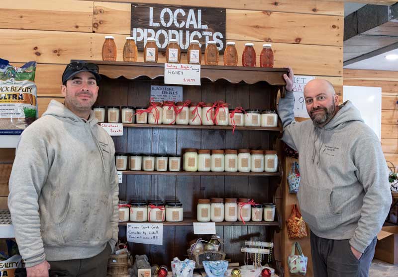
Mike Hood (still left) and Rob Hood stand in entrance of a Blackstone Candle screen at Three Seasons Garden Shop.  (Photograph by Thomas Kilian)

Mike, Rob, and their four siblings all grew up on Aged Mill Highway immediately after their mom and dad moved there 47 several years ago. Their father, Bob Hood, sent the mail in town for 25 decades, and their maternal grandmother, Rita Lombardi, was celebrated at the 2018 City Assembly as the town’s oldest resident. She died at household in 2021 at the age of 102.

Looking again and reflecting on her sons’ achievements, Peggy Hood advised the Press she wasn’t astonished when her outside-loving sons Mike and Tim took up landscaping as a career. All through their youth, she’d line up outside assignments for them at their Grandfather Lombardi’s spot in Clinton. He was an engineer by occupation, but in retirement targeted on meticulous lawn and stone get the job done. “He was exacting and taught them a ton,” she claimed. To this working day, she reported, “Mike prefers to be out and about.”

Rob, also, is well suited to his existing job in the Three Seasons business, controlling the workplace and inventory at the keep and creating up proposals for landscaping customers. He “always preferred books and is extremely clever … they are a very good match for the enterprise,” Peggy mentioned.

The retail enterprise started with the sale of mums on the store’s garden in 2020, though the store itself opened in the spring of 2021—after the previous storage building had been renovated. It was paneled in knotty pine milled at a Hubbardston lumber mill, and the partitions were being adorned with antique farm implements that the Hoods discovered in an old barn on the residence. Among 2021 and 2022, stock at the shop steadily enhanced. Currently, the shop carries backyard tools of all varieties flower pots grass seed, backyard garden soil, and soil amendments and gift objects, which include Blackstone candles and diminutive, handmade reward bags. Seasonal things these as bushes and flowering crops mulch, pumpkins, and hay bales and Xmas trees, wreaths, and arrangements make appearances throughout the months the keep is open, which are April 1 by way of Christmas.

Reflecting on the previous yr, Mike says he has experienced the most entertaining selling Xmas trees, and if he had to opt for a preferred solution, he’d go with the Jonathan Environmentally friendly grass seed, which he swears by. The opening future 12 months of a further backyard garden middle on Ayer Road—just as the retailer gains steam—has the two Rob and Mike established to retain improving 3 Seasons. Up coming year, for instance, Mike designs to develop the inventory to include wild chook supplies, perennials, seeds, organic double-ground mulch, stone, and substantial-conclusion outside hearth units from Montana Fireplace Pits.

Property developer exploring mining possibilities at seaside beauty spot

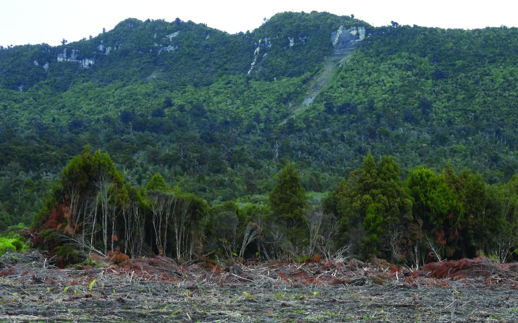
The Rapahoe block, with work under way below the Twelve Apostles Range.

The Rapahoe block, with function beneath way under the Twelve Apostles Selection.
Photograph: Brendon McMahon / Greymouth Star

A distinguished 16ha block bordering the seaside settlement of Rapahoe and State Highway 6 could be subdivided into way of life-measurement residential blocks.

However, developer Terry Birchfield states he is also checking out the risk of mining the web site, which has a spectacular Twelve Apostles Selection backdrop.

Tall flax and scrub and some bush re-growth has been flattened or cleared and new drains fashioned given that Birchfield acquired the assets previously this yr.

Fox River resident Andrew Beaumont contacted the Greymouth Star involved that function might be destroying what appeared to be a normal wetland.

“They are chopping into that regrowth of bush and placing in drains,” he mentioned. “It seems to me like a pretty massive indigenous wetland space that could be appeared following.”

However, Birchfield stated the block was not naturally swampy, even with passing impressions. Run-off from the adjacent freeway intended water experienced nowhere else to go.

“The street drain runs across into our location and there is no drain managing away from it, and it is really created a bloody mess of it. The road board (NZTA) is growling at me. We’re getting the water from the other side of the highway.”

The internet site alone experienced great normal drainage on sand, about 1m to 1.5m beneath the prime layer of soil, he stated.

The foreseeable future subdivision would be serviced with electricity and linked to drinking water, becoming near to services in Runanga and Rapahoe.

Any progress was a pretty “gradual task” but the land was appealing for subdivision supplied its proximity to the coastline.

At the very same time, test sampling for possible sand-primarily based mineral content experienced been carried out.

“You will find all sorts of minerals close to these days. Gold is a person of them, but we’re all a bit ahead of our time,” Birchfield stated.

West Coastline Regional Council acting consents and compliance supervisor Rachel Clark stated the council was aware of preliminary perform for some kind of potential progress along Rapahoe straight.

“We are examining it, and we want to glimpse into it. I think they ended up undertaking most of what they were being undertaking less than permitted activity rules.”

Gray District Council senior planner Michael McEnaney claimed the web site was not an discovered important normal location in the district prepare. Nor experienced it been discovered as an outstanding natural landscape or an spot of large normal character inside of the proposed Te Tai o Poutini Strategy.

The NZ Transportation Company has been approached for comment.

Local Democracy Reporting is Community desire journalism is funded by NZ on Air

If there is a film on Four Seasons Total Landscaping, remember you read it here first!

The Black Listing is an yearly listing that names the most popular unproduced screenplays in Hollywood. The listing was first posted in 2005 by Franklin Leonard, a growth government who at the time worked for Overbrook Leisure, the output corporation cofounded by Will Smith and named for his West Philadelphia community.

The Black Record is assembled from a survey of Hollywood producers and other final decision-makers, who vote on the prime unproduced scripts they have study in the very last yr. Argo, The King’s Speech, Slumdog Millionaire, and Spotlight are some of the list’s shining alums. 2013′s American Hustle, a fictionalized variation of the Philadelphia-linked Abscam scandal, has also been on the record.

This year’s Black Listing arrived Dec. 12 and bundled a screenplay about a single of the most talked-about events to get spot in Philadelphia in the last number of decades.

The script, known as Total Landscaping, purports to notify the story of that day in November 2020 when Donald Trump’s presidential marketing campaign, led by Rudy Giuliani, inexplicably held a news conference exterior of Four Seasons Complete Landscaping, a relatives-owned landscaping small business in Northeast Philadelphia. For the duration of the news meeting, held in a strip shopping mall that also involved a crematorium and a intercourse store, the main networks named Pennsylvania and the election for Joseph Biden.

Given that then, the Full Landscaping site has come to be a well-known destination, and the firm had merchandise revenue reportedly totaling $1.3 million.

The Whole Landscaping script is credited to Woody Bess. For each the description, the screenplay describes “a day in the existence of the employees of 4 Seasons Full Landscaping and its neighboring organizations on November 7th, 2020: the day an normal, operating-course strip mall in East Philadelphia [sic] turned the focal position of the most divisive presidential election in American Record.”

Ought to we be wanting to know what tack the eventual movie may possibly consider, irrespective of whether it will be filmed locally, or who may be forged as Giuliani in his most outstanding film overall look considering that Borat Subsequent Moviefilm?

Almost certainly not, at least not for a although.

Bess, the writer, is a Massachusetts indigenous and USC grad, who is now directing a film and was not out there for a comment. The Inquirer spoke to his supervisor, Jeff Portnoy, who is credited in the Black List listing.

Portnoy described the script as “more impressed by a genuine tale, than a accurate tale,” and that it was based mostly on intensive research accomplished by Bess. The script has not but been optioned, bought, or taken any other actions toward getting to be a movement picture. In simple fact, it could not turn out to be a film at all.

Portnoy described that the Overall Landscaping script is what is acknowledged as a “stunt spec.” That’s when a author writes a script, usually of a Tv series episode (but also in some cases a motion picture), in which the target is not so a lot for the movie to be produced than for producers, agents, or studios to discover the writer’s talent and seek the services of that particular person to write a thing else.

The strategy, Portnoy claimed, was to “put them on the map, and make a enjoyable read through for the market … they get standard meetings out of it and get agency illustration.”

This was the case with the 2019 Black Checklist script Barron: A Tale of Like, Loss & Legacy, which spun an imaginative tale out of a then-10-calendar year-aged Barron Trump sabotaging his dad’s operate for president. That film, for many and obvious good reasons, was never manufactured, but its author has considering that gotten studio function.

The Complete Landscaping script, Portnoy claimed, is a little bit “more producible.”

The screenplay was not prepared with the cooperation of the men and women who own Whole Landscaping, but Portnoy said that should a important producer or studio come along, they would talk with the business’ owners.

Four Seasons Total Landscaping did not answer to an e mail requesting remark.

The 2021 documentary 4 Seasons Total Documentary debuted on MSNBC on the to start with anniversary of the working day in dilemma. And the footage from that working day is set to seem in a lot of long term documentaries about the 2020 election.

Binding affinity estimation from restrained umbrella sampling simulations

Theoretical foundation

Binding affinity is often quantified using the equilibrium dissociation constant (Kd), defined as:

$$K_mathrmd = left[ mathrmP right]left[ mathrmL right]/left[ mathrmP:mathrmL right]$$

(1)

where [P], [L] and [P:L] are the concentrations of protein, ligand and the protein–ligand complex, respectively. Computationally, the absolute binding free energy (ΔG°), which is the standard molar free energy of binding, is more convenient to calculate. The dissociation constant and the absolute binding free energy are related via

$$Delta G^circ = RTln fracK_mathrmd1,mathrmM$$

(2)

where R is the gas constant, T is the temperature and 1 M is 1 molar concentration. Various strategies have been used to estimate ΔG°, some of which were briefly discussed above. The methodology proposed here has a notable resemblance to the stratification strategy of refs. 3,4. However, the two methods have major differences as will be discussed later in this section.

Absolute binding free energy or ΔG° is the free-energy change associated with moving the ligand from the bulk to the binding pocket (Supplementary Table 1). Within the formalism presented in this work, ΔG° is determined from the grid PMF G(x), where x is the position of the ligand mass center from the center of the binding pocket (Supplementary Table 1), G(x) is the PMF associated with the ligand position x. In practice, we need to bin the three-dimensional space and define the PMF at every bin or grid point as:

$$Gleft( boldsymbolx right) = – RTln pleft( boldsymbolx right)$$

(3)

where p(x) is the probability of finding the ligand at bin x.

We define ΔG(x) = G(x) − G(0), where x = 0 (that is, the center of the binding pocket) is defined as the grid point associated with the lowest grid PMF. One can show:

$$Delta G^circ = – RTln frac{{int_mathrmpocket {mathrme^ – fracGleft( boldsymbolx right)RT} mathrmdV}}{{int_mathrmbulk {mathrme^{ – frac{Gleft( boldsymbolx right)}RT}} mathrmdV}} = – RTln frac{{int_mathrmpocket {mathrme^ – fracDelta Gleft( boldsymbolx right)RT} mathrmdV}}{{int_mathrmbulk {mathrme^ – fracDelta Gleft( boldsymbolx right)RT} mathrmdV}}$$

(4)

in which the binding ‘pocket’ refers to all xV where the ligand is considered bound and ‘bulk’ refers to all xV where the ligand is not interacting with the protein. V here is a subset of space with a single protein in standard concentration (that is, 1 M). As ΔG(x) is the same everywhere in the bulk, we can simplify relation (4) as follows:

$$Delta G^circ = – RTln fracV_mathrmP{{mathrme^{ – frac{Delta Gleft( boldsymbolx_mathrmB right)}RT}V_mathrmB}} = – Delta Gleft( boldsymbolx_mathrmB right) – RTln fracV_mathrmPV_mathrmB$$

(5)

where VB is the bulk volume per protein associated with the standard concentration, xB is any grid point in the bulk and VP is the binding pocket volume defined as:

$$V_mathrmP = mathop intnolimits_mathrmpocket {mathrme^{ – fracDelta Gleft( boldsymbolx right)RT}} mathrmdV$$

(6)

Defining ΔGV as the contribution of the difference between the volume of the binding pocket and the bulk to the binding free energy:

$$Delta G_mathrmV = – RTln fracV_mathrmPV_mathrmB$$

(7)

Combining equations (5) and (7), we have:

$$Delta G^circ = – Delta Gleft( boldsymbolx_mathrmB right) + Delta G_mathrmV$$

(8)

We can find the bulk volume (VB) associated with the standard concentration for a single protein approximately as:

$$V_mathrmB = frac{frac1N_mathrmA,mathrmmol}{1,mathrmM} = frac1{N_mathrmA}mathrmL approx 1,661,mathrmAA^3$$

(9)

where NA is Avogadro’s constant and L is the unit of volume (litres). We can now rewrite ΔGV as:

$$Delta G_mathrmV = – RTln fracV_mathrmPV_mathrmB = – RTln frac{V_mathrmP}mathrmAA^3 + RTln fracV_mathrmBmathrmAA^3 = Delta G_mathrmP – Delta G_mathrmB$$

(10)

in which ΔGB is the bulk volume contribution and ΔGP is the binding pocket contribution:

$$left{ {beginarray*20l {Delta G_mathrmB = – RTln frac{{V_mathrmB}}{mathrmAA^3} approx – 7.42RT} hfill \ {Delta G_mathrmP = – RTln frac{{V_mathrmP}}{{mathrmAA^3}} = – RTln mathop intnolimits_mathrmpocket {mathrme^{ – frac{Delta Gleft( boldsymbolx right)}RT}} fracmathrmdV{{mathrmAA^3}}} hfill endarray} right.$$

(11)

Determining both ΔG(xB) and ΔGP requires finding the grid PMF ΔG(x). ΔG(xB) is the PMF difference between the binding pocket center and the bulk and ΔGP also requires an estimate for ΔG(x) within the binding pocket. We therefore do not need to find ΔG(x) for all x if we have a good estimate for ΔG(x) within the binding pocket and in the bulk. Ideally, ΔG(x) for these points can be determined by pulling the ligand out of the binding pocket towards the bulk and using an enhanced sampling technique such as US to sample the space of a collective variable such as d, that is, the distance between the mass centers of the ligand and protein. ΔG(x) can be estimated for all sampled grid points x using this distance-based US simulation. Note that the collective variable used for biasing would be d, while the collective variable used for the PMF calculations would be the three-dimensional position vector of the mass center of ligand with respect to protein’s binding pocket center. One may estimate the grid PMF from the distance-based US simulations using a non-parametric reweighting algorithm as discussed in this section. ΔG(x) can also be used to estimate ΔGP as defined in relation (11). There is often no need to strictly define the binding pocket as only low ΔG(x) values have non-negligible contribution to VP and thus even if we include all sampled grid points, only those close to the binding pocket center have non-negligible contributions.

A practical issue with determining ΔG(xB) is the convergence. The key obstacles for the sampling that slow down the convergence are the orientation of the ligand, and the conformational changes of the ligand and protein. Using an approach similar in spirit to the previously proposed stratification strategy3,4,24, we can circumvent extensive sampling of these degrees of freedom. Let us first focus on the orientation of the ligand (Ω), defined using the orientation quaternion formalism. We can restrain Ω during the distance-based US simulations using a biasing potential ((frac12kvarOmega ^2) where a k is harmonic force constant) and later correct the free-energy difference based on the PMF associated with the Ω, which is different in the bulk (F(xB, Ω)) and in the binding pocket (F(0, Ω)). More generally, for any grid point x, we may determine ΔG(x) based on the PMF associated with the Ω at x (F(x, Ω)) and 0 (F(0, Ω)):

$$mathrme^ – fracDelta G(boldsymbolx)RT = frac{{int_!0^uppi {mathrme^ – fracF(boldsymbolx,varOmega )RTmathrmdvarOmega } }}{{int_!0^uppi {mathrme^ – fracF(boldsymbol0,varOmega )RTmathrmdvarOmega } }}$$

(12)

Note that F(x, Ω) is the PMF associated with x and Ω, defined such that:

$$Gmathrm(boldsymbolxmathrm) = c – RTln mathop intnolimits_!0^uppi {mathrme^{ – fracF(boldsymbolx,varOmega )RT}mathrmdvarOmega }$$

(13)

where c is an arbitrary constant. We therefore have:

$$mathrme^{ – frac{Delta G(boldsymbolx)}RT} = frac{{int_!0^uppi {mathrme^{ – frac{F(boldsymbolx,varOmega )}RT}mathrmdvarOmega } }}{{int_!0^uppi {mathrme^ – fracF(boldsymbolx,varOmega ) + frac12kvarOmega ^2RTmathrmdvarOmega } }} times frac{{int_!0^uppi {e^ – fracF(boldsymbol0,varOmega ) + frac12kvarOmega ^2RTmathrmdvarOmega } }}{{int_!0^uppi {e^{ – fracF(boldsymbol0,varOmega )RT}mathrmdvarOmega } }} times frac{{int_!0^uppi {mathrme^{ – fracF(boldsymbolx,varOmega ) + frac12kvarOmega ^2RT}mathrmdvarOmega } }}{{int_!0^uppi {mathrme^{ – frac{F(boldsymbol0,varOmega ) + frac12kvarOmega ^2}RT}mathrmdvarOmega } }}$$

(14)

We now define GΩ(x) as the grid PMF of the restrained system (by Ω):

$$G_varOmega (boldsymbolx) = – RTln mathop intnolimits_!0^uppi {mathrme^{ – frac{F(boldsymbolx,varOmega ) + frac12kvarOmega ^2}RT}mathrmdvarOmega }$$

(15)

We also define UΩ(x) as the average biasing potential at grid point x:

$$U_varOmega left( boldsymbolx right) = – RTln langle mathrme^ – fracfrac12kvarOmega ^2RT rangle _boldsymbolx = – RTln frac{{int_0^uppi {mathrme^{ – frac{{Fleft( boldsymbolx,varOmega right) + frac12kvarOmega ^2}}RT}} mathrmdvarOmega }}{{int_0^uppi {e^{ – frac{{Fleft( boldsymbolx,varOmega right)}}RT}} mathrmdvarOmega }}$$

(16)

Now we have from relations (14), (15) and (16):

$$Delta Gleft( boldsymbolx right) = Delta G_varOmega left( boldsymbolx right) – Delta U_varOmega left( boldsymbolx right)$$

(17)

where, the free energy of grid point x from the center 0G(x)) is calculated based on its equivalent free energy (ΔGΩ(x)) in a system biased by a harmonic restraint on Ω and a correction term ΔUΩ(x). For x = xB:

$$Delta U_varOmega left( boldsymbolx_mathrmB right) = – RTln frac{{langle mathrme^ – fracfrac12kvarOmega ^2RT rangle _mathrmbulk}}{{langle mathrme^ – fracfrac12kvarOmega ^2RT rangle _mathrmpocket}}$$

(18)

To determine the above ensemble averages, we need to determine the PMF along Ω for the bound and unbound ligand and calculate the ensemble averages analytically using relation (16). ΔGΩ(xB) can be determined from PMF calculations, where the distance between the protein and ligand is varied and the orientation of the ligand is restrained (distance-based BEUS with restrained orientation). We note that:

$$V_mathrmP = mathop intnolimits_mathrmpocket {mathrme^{ – frac{{Delta Gleft( boldsymbolx right)}}RT}} mathrmdV = mathop intnolimits_mathrmpocket {mathrme^{ – frac{Delta G_varOmega left( boldsymbolx right) – Delta U_varOmega left( boldsymbolx right)}RT}} mathrmdV approx mathop intnolimits_mathrmpocket {mathrme^{ – frac{Delta G_varOmega left( boldsymbolx right)}RT}} mathrmdV$$

(19)

where we assume ΔUΩ(x) is negligible for x within the binding pocket. In other words, (langle {mathrme^ – fracfrac12kvarOmega ^2RT} rangle _boldsymbolx approx langle {mathrme^ – fracfrac12kvarOmega ^2RT} rangle _boldsymbol0) for x close to 0.

In brief, if we choose to restrain the orientation, our absolute binding-free-energy estimate includes the following terms (using relations (8) and (17)):

$$Delta G^circ = – Delta G_varOmega left( boldsymbolx_mathrmB right) + Delta U_varOmega left( {boldsymbolx_mathrmB} right) + Delta G_mathrmV$$

(20)

F(xB, Ω) can be calculated numerically from orientation angle distribution of a free ligand: (F(boldsymbolx_mathrmB,varOmega ) = – RTln pleft( varOmega right),) where p(Ω) is determined from the distribution of Euler angles ((pleft( phi ,theta ,psi right) = frac18uppi ^2sin theta), where 0 ≤ ϕ, ψ ≤ 2π and 0 ≤ θ ≤ π) given that:

$$cos fracvarOmega 2 = cos fracphi 2cos fractheta 2cos fracpsi 2 + sin fracphi 2sin fractheta 2sin fracpsi 2$$

(21)

(langle {mathrme^ – fracfrac12kvarOmega ^2RT} rangle _{mathrmbulk}) can then be calculated using relation (16) with numerically estimated F(xB, Ω) and the k value used in the simulations. (Fleft( {boldsymbolx_mathrmB,varOmega } right) = – RTln p(varOmega )) was numerically estimated by discretizing each of the 3 Euler angles with a bin width of 1° and a total of 360 × 360 × 180 bins to estimate p(Ω) from p(ϕ, θ, ψ). F(0, Ω) can be determined approximately using orientation-based US simulations of bound ligand. F(0, Ω) can then be used to estimate (langle {mathrme^{ – fracfrac12kvarOmega ^2RT}} rangle _mathrmpocket) using relation (16).

The above strategy can be extended to other degrees of freedom for which unbiased sampling may hinder the convergence. Most notably, the internal conformational changes of the ligand and that of the protein may also play a crucial role in slowing down the convergence. In the following, we show how one can restrain not only the orientation of the ligand but also the RMSD of the ligand (denoted here by r) in distance-based US simulations (along d) to speed up convergence. In this case, the grid PMF difference ΔG(x) is calculated based on ΔGΩ,r(x), the grid PMF of a system whose Ω and r are both restrained:

$$mathrme^{ – frac{{Delta Gleft( boldsymbolx right)}}RT} = frac{{int_!0^infty {int_0^uppi {mathrme^{ – frac{{Fleft( {boldsymbolx,varOmega ,r} right)}}RT}} } mathrmdvarOmega mathrmdr}}{{int_!0^infty {int_!0^uppi {mathrme^{ – fracFleft( boldsymbol0,varOmega ,r right)RT}} } mathrmdvarOmega mathrmdr}}$$

(22)

Using a similar strategy as in relation (14), we have:

$$beginarraylmathrme^ – fracDelta Gleft( x right)RT = frac{{mathop smallint nolimits_0^infty mathop smallint nolimits_0^uppi mathrme^{ – frac{{Fleft( {boldsymbolx,Omega ,r} right)}}RT}mathrmdvarOmega mathrmdr}}{{mathop smallint nolimits_0^infty mathop smallint nolimits_0^uppi mathrme^{ – frac{{Fleft( {boldsymbolx,varOmega ,r} right) + frac12k^prime r^2}}RT}mathrmdvarOmega mathrmdr}} times frac{{mathop smallint nolimits_0^infty mathop smallint nolimits_0^uppi mathrme^{ – frac{{Fleft( {boldsymbolx,varOmega ,r} right) + frac12k^prime r^2}}RT}mathrmdvarOmega mathrmdr}}{{mathop smallint nolimits_0^infty mathop smallint nolimits_0^uppi mathrme^{ – frac{{Fleft( {boldsymbolx,varOmega ,r} right) + frac12k^prime r^2 + frac12kvarOmega ^2}}RT}mathrmdvarOmega mathrmdr}}\ times frac{{mathop smallint nolimits_0^infty mathop smallint nolimits_0^uppi mathrme^ – fracFleft( 0,varOmega ,r right) + frac12k^prime r^2 + frac12kvarOmega ^2RTmathrmdvarOmega mathrmdr}}{{mathop smallint nolimits_0^infty mathop smallint nolimits_0^uppi mathrme^{ – fracFleft( boldsymbol0,varOmega ,r right) + frac12k^prime r^2RT}mathrmdvarOmega mathrmdr}} times frac{{mathop smallint nolimits_0^infty mathop smallint nolimits_0^uppi mathrme^{ – frac{{Fleft( boldsymbol0,varOmega ,r right) + frac12k^prime r^2}}RT}mathrmdvarOmega mathrmdr}}{{mathop smallint nolimits_0^infty mathop smallint nolimits_0^uppi mathrme^{ – frac{{Fleft( boldsymbol0,varOmega ,r right)}}RT}mathrmdvarOmega mathrmdr}}\ times frac{{mathop smallint nolimits_0^infty mathop smallint nolimits_0^uppi mathrme^{ – frac{{Fleft( {boldsymbolx,varOmega ,r} right) + frac12k^prime r^2 + frac12kvarOmega ^2}}RT}mathrmdvarOmega mathrmdr}}{{mathop smallint nolimits_0^infty mathop smallint nolimits_0^uppi mathrme^{ – frac{Fleft( boldsymbol0,varOmega ,r right) + frac12k^prime r^2 + frac12kvarOmega ^2}RT}mathrmdvarOmega mathrmdr}}endarray$$

(23)

which results in:

$${rme^{ – fracDelta Gleft( bfx right)RT}} = frac{{{{langle {rme^ – fracfrac12k^prime r^2RT}rangle }_bf0}}}{{{{langle {rme^{ – fracfrac12k^prime r^2RT}}rangle }_bfx}}} times frac{{{{langle {rme^{ – fracfrac12kvarOmega ^2RT}}rangle }_}0^r}}{{langle {rme^{ – frac{{frac12kvarOmega ^2}}RT}}rangle _bfx^r}} times frac{{rme^ – beta G_varOmega ,r(bfx)}}{{rme^ – beta G_varOmega ,r(bf0)}}$$

(24)

Here we have defined GΩ,r(x) as:

$$G_varOmega ,rleft( boldsymbolx right) = – RTln mathop intnolimits_0^infty {mathop intnolimits_0^uppi {mathrme^{ – frac{{Fleft( {boldsymbolx,varOmega ,r} right) + frac12k^prime r^2 + frac12kvarOmega ^2}}RT}} }$$

(25)

where k′ is the harmonic force constant associated with the r based on biasing potential ((frac12k^prime r^2)). We also define Ur(x) similar to UΩ(x) in relation (15) except for using r instead of Ω. (U_varOmega^r(boldsymbolx)) is also defined similar to UΩ(x) except for the additional restraint on r:

$$U_varOmega ^rleft( x right) = – RTln langle {mathrme^{ – frac{{frac12kvarOmega ^2}}RT}} rangle _boldsymbolx^r = – RTln frac{{mathop smallint nolimits_0^infty mathop smallint nolimits_0^uppi mathrme^{ – frac{{Fleft( {boldsymbolx,varOmega ,r} right) + frac12k^prime r^2 + frac12kvarOmega ^2}}RT}mathrmdvarOmega mathrmdr}}{{mathop smallint nolimits_0^infty mathop smallint nolimits_0^uppi mathrme^{ – frac{{left( {Fleft( {boldsymbolx,varOmega ,r} right) + frac12k^prime r^2} right)}}RT}mathrmdvarOmega mathrmdr}}$$

(26)

Finally, we have:

$$Delta Gleft( boldsymbolx right) = Delta G_{varOmega ,r}left( {boldsymbolx} right) – Delta U_rleft( {{{boldsymbolx}}} right) – Delta U_{varOmega }^rleft( {{{boldsymbolx}}} right)$$

(27)

In brief, if we choose to restrain both the orientation and RMSD, our absolute binding-free-energy estimate includes the following terms:

$$Delta G^circ = – Delta G_varOmega ,rleft( {{{{boldsymbolx}}}_mathrmB} right) + Delta U_rleft( {{{{boldsymbolx}}}_mathrmB} right) + Delta U_varOmega ^rleft( {{{{boldsymbolx}}}_mathrmB} right) + Delta G_mathrmV$$

(28)

Here we are using an approximation similar to that in relation (19):

$$V_mathrmP approx mathop intnolimits_mathrmpocket {mathrme^{ – frac{{{{Delta }}G_{{{varOmega }},r}left( {{{boldsymbolx}}} right)}}{RT}}} mathrmdV$$

(29)

Using relations (20) and (28), we can generalize the stratification strategy to include three restraints on arbitrary collective variables α, β and γ:

$$Delta G^circ = – Delta G_alpha ,beta ,gamma left( {{{{boldsymbolx}}}_mathrmB} right) + Delta U_gamma left( {{{{boldsymbolx}}}_mathrmB} right) + Delta U_beta ^gamma left( {{{{boldsymbolx}}}_mathrmB} right) + Delta U_alpha ^beta ,gamma left( {{{{boldsymbolx}}}_mathrmB} right) + Delta G_mathrmV$$

(30)

where:

$$Delta G_mathrmV approx – RTln mathop intnolimits_{{mathrmpocket}} {mathrme^{ – frac{{Delta G_alpha ,beta ,gamma ({{{boldsymbolx}}})}}{{RT}}}} frac{mathrmdV}{{{mathrmAA}^3}} – Delta G_mathrmB$$

(31)

Isothermal titration calorimetry of hFGF1 with heparin hexasaccharide

ITC data were obtained using MicroCal iTC 200 (Malvern) with microcal origin software. The change in heat during the biomolecular interaction was measured by titrating heparin (loaded in the syringe) into the hFGF1 solution in the calorimetric cell. Both the protein and the heparin samples were prepared in the buffer containing 10 mM phosphate buffer with 100 mM NaCl at pH 7.2 and were degassed before loading. The protein-to-heparin ratio was maintained at 1:10 with the protein concentration being 100 μM and the heparin concentration being 1 mM. A total of 30 injections were conducted with a constant temperature of 25 °C and stirring speed of 300 rpm. One set of sites binding model was used for the ITC binding curve68. The standard binding free energy ΔG° was determined from dissociation constant via relation (2) at T = 25 °C. The experiment was repeated three times with the same sample and the results obtained were very similar to each other. The mean and standard deviation were reported for both Kd and ΔG°.

All-atom MD simulations

For our bound state, we utilized the X-ray crystal structure of the dimeric hFGF1 combination with heparin hexasaccharide (PDB 2AXM; resolution, 3.0 Å)69, and for our apo state, we used the X-ray crystal structure of monomeric hFGF1 (PDB 1RG8; resolution, 1.1 Å)70. The NAMD 2.13 (ref. 71) was used to run MD simulations. Using a conjugate gradient, we energy-minimized the system for 10,000 steps. We next relaxed the systems using stepwise restrained MD simulations (for 1 ns) using CHARMM-GUI72. All production runs were done in an NPT (constant N, number of atoms; P, pressure; T, temperature) ensemble after the first NVT (constant N, number of atoms; V, volume; T, temperature) relaxation. Simulations were done at 300 K with a 2 fs time step and a 0.5 ps−1 damping coefficient using a Langevin integrator. Nosé–Hoover–Langevin pistons were used to maintain 1 atm pressure72. Long-range electrostatic interactions were estimated using the particle mesh Ewald approach. The initial runs were done for 15 ns, followed by the production run on the Anton 2 supercomputer (Pittsburgh Supercomputing Center) for 4.8 μs with a 2.5 fs time step.

MD simulations of free heparin hexasaccharide

Heparin hexasaccharide69 was simulated in a rectangular water box without the protein. The system was set up as described previously in the ‘All-atom MD simulations’ section. The final conformation after relaxation was then used as the starting conformation for 10 production runs for 40 ns each. The total simulation time was around 400 ns.

SMD simulations

The final conformations of the hFGF1–heparin73, apo hFGF1 (ref. 73) and free heparin hexasaccharide equilibrium simulations were used to generate starting conformations for the non-equilibrium pulling simulations. Four collective variables74 were used for the SMD simulations75: (1) distance between the heavy-atom center of mass of heparin and that of the protein (d); (2) the orientation angle of heparin with respect to the protein (Ω) defined using the orientation quanternion formalism; (3) RMSD of the protein (rP); (4) RMSD of heparin (rL). Six independent sets of simulations were performed. The distance-based SMD simulation was run for 9.5 ns, while the orientation-based SMD simulation was run for 8 ns. The distance-based SMD simulation was used to pull the heparin away from the protein by approximately 30 Å (10 Å  40 Å) with a force constant of 100 kcal (mol Å2)−1. The orientation angle was also restrained in this simulation with a force constant of 0.5 kcal (mol degree2)−1 to stay close to its initial orientation in the bound state. The orientation-based SMD simulation was used to rotate the bound heparin locally with respect to the protein (0° → 73°) with a force constant of 100 kcal (mol degree2)−1. Four RMSD-based SMD simulations were run for 10 ns each using a force constant of 50 kcal (mol Å2)−1: (1) to change the RMSD of the bound protein (0.5 Å→2 Å) (the RMSD of heparin was restrained in this simulation with a force constant of 1 kcal (mol Å2)−1); (2) to change the RMSD of the bound heparin (1.5 Å → 4 Å); (3) to change the RMSD of the unbound protein (0.8 Å → 3.2 Å); (4) to change the RMSD of the free heparin (1.5 Å → 5.5 Å).

BEUS simulations

BEUS53,76,77, which is a variation of the US simulation method, was performed to estimate grid PMF (Supplementary Fig. 1). Four independent sets of distance (d)-based BEUS simulations were performed, with no restraints, restraint on orientation angle of heparin with respect to the protein (Ω), restraint on RMSD of the ligand (rL) and RMSD of the protein (rP), and restraints on Ω, rL and rP. Two sets of BEUS simulations were also performed using the Ω collective variable, one with and one without a restraint on rL and rP. In addition, two sets of BEUS simulations were performed using the rP collective variable (bound protein with restraint on rL; unbound protein) and two sets were performed using the rL collective variable (bound ligand; free ligand). Selected SMD conformations were assigned to individual BEUS windows with equal spacing in each one of these BEUS simulations. The distance-based BEUS simulations ran for 10 ns with 31 replicas/windows and the orientation-based simulations ran for 10 ns with 30 replicas/windows. The RMSD-based BEUS simulations ran for 10 ns with 12 replicas/windows. The force constant used for ligand–protein distance (d) in distance-based BEUS was 2 kcal (mol Å2)−1 while the orientation was restrained as in SMD simulations using a force constant of 0.5 kcal (mol degree2)−1. For orientation-based BEUS simulations, the force constant for the ligand orientation angle (as in SMD simulations) was set to 0.5 kcal (mol degree2)−1. The force constant used for rL and rP in all cases was 1 kcal (mol Å2)−1. See Supplementary Fig. 1 for a schematic representation of these simulations.

Free-energy calculations using non-parametric reweighting

Once the BEUS simulations described above were converged, a non-parametric reweighting method76,78, which is somewhat similar to the multi-state Bennett acceptance ratio method79, was used to construct the PMF. In this method76, each sampled configuration will be assigned a weight, which can be used to construct the PMF in terms of a desired collective variable. Suppose that a system is biased (for instance, within a BEUS scheme) using N different biasing potentials Ui(r), where i = 1, …, N, and r represents all atomic coordinates. Typically, Ui(r) is a harmonic potential defined in terms of a collective variable with varying centers for different i. Assuming an equal number of sampled configurations from each of the N generated trajectories, we can combine them in a single set of samples rk (irrespective of which bias was used to generate each sample rk) and determine the weight of each sample (wk) as:

$$w_k = c/mathop sumlimits_i {mathrme^{ – frac{{left( {U_ileft( boldsymbolr_k right) – F_i} right)}}{{RT}}}}$$

(32)

where, c is the normalization constant such that (mathop sumnolimits_k w_k = 1) and both wk and perturbed free energies Fi are determined iteratively using the above equation and the following:

$$mathrme^ – beta F_i = mathop sumlimits_k {w_kmathrme^{ – frac{{U_ileft( boldsymbolr_k right)}}{{RT}}}}$$

(33)

Converged wk values can be used to construct any ensemble averages including any PMF (for example, G(ζ) PMF of the atomic system in the collective variable space(ζ))) in terms of not only the collective variable used for biasing but also any other collective variables that are sufficiently sampled. One may use a weighted histogram method to construct the PMF as follows:

$$Gleft( boldsymbolupzeta _i right) = – RTln mathop sumlimits_k w_k delta left( {boldsymbolupzeta left( {boldsymbolr_k} right) – boldsymbolupzeta _i} right),$$

(34)

$$delta left( {boldsymbolupzeta left( {{{boldsymbolr}}_k} right) – boldsymbolupzeta _i} right) = left{ {beginarray*20l 1, hfill & {left| {boldsymbolupzeta left( {{{{boldsymbolr}}}_k} right) – {{boldsymbolupzeta }}_i} right| < left| {{{{boldsymbolupzeta }}}left( {{{{boldsymbolr}}}_k} right) – {{{boldsymbolupzeta }}}_j} right|mathrmfor,j ne i.} hfill \ 0, hfill & mathrmotherwise hfill endarray} right.$$

(35)

To estimate the uncertainty of any of PMF calculations described above, one may use bootstrapping. Here, we have used a block Bayesian bootstrapping technique77, where 100 alternative datasets are resampled from the existing dataset and the same non-parametric reweighting algorithm and the same PMF calculation is repeated for each set to generate 100 alternative PMFs. The standard deviation of the PMF at any point along the reaction coordinate provides an estimate for the error.

Alchemical FEP simulations

We used the BFEE2 (ref. 27) package to estimate the absolute free energy of binding in silico for an alchemical or geometrical route with multiple subprocesses and geometric constraints. Alchemical FEP simulations were performed to calculate the absolute binding free energy for the interaction of hFGF1 with heparin hexasaccharide. We used a double annihilation protocol80, wherein the heparin hexasaccharide is annihilated in both the free and bound states. The final conformations of the hFGF1–heparin complex73 and free heparin hexasaccharide equilibrium simulations (discussed previously in the ‘All-atom MD simulations’ section) were used to generate starting conformations for the bound hFGF1–heparin and free heparin FEP simulations respectively. For the alchemical route, four separate simulations are performed: (1) coupling the restraints of seven collective variables in the bound state; (2) decoupling the ligand alchemically in the bound state; (3) coupling the ligand alchemically in the unbound state; (4) decoupling the conformational restraints in the unbound state. The FEP simulations 1 and 3 were performed bidirectionally using 200 λ-windows (λ is the coupling parameter associated with the FEP that could vary between 0 and 1). Each λ-window included a 0.5 ns of equilibration and 5.0 ns of averaging for both the unbound and bound states, for a total of 2.3 μs (Supplementary Table 3). The decoupling FEP simulations 2 and 4 were also performed bidirectionally, each one for 51 ns. All FEP simulations were performed using the NAMD 2.13 (ref. 71) simulation package with the CHARMM36m all-atom additive force field, using the protocol discussed previously for the equilibrium simulations. We used the state-of-the-art BFEE2 (ref. 27) method to make input files and analyze the FEP simulations.

Binding-free-energy calculations using geometrical route

The extended ABF technique with an umbrella integration estimator was used to calculate the free-energy change along the coarse variables required to characterize reversible heparin–hFGF1 binding3,24,27. We used the software BFEE2 (ref. 27) to generate the input files for these simulations. In the geometrical route, these collective variables are often subjected to restrictions, and the amount of reversible work required to impose each constraint is determined by a sequence of very accurate PMF simulations. The collective variables used here are the RMSDs of the two proteins’ backbone distances from the reference, native conformation, the three Euler angles (Θ, Φ and Ψ) that describe their relative orientation and the polar (θ) and azimuth angles (φ) that describe their relative position27,81. The geometrical path consists of a sequence of separate PMF computations performed sequentially with the gradual inclusion of restrictions (RMSD, Θ, Φ, Ψ, θ and φ), as shown in Supplementary Table 2. Each geometric collective variable (RMSD, Θ, Φ, Ψ, θ, φ and r = (1/β) ln(S*I*C°); β = (𝑘BT)−1, with kB the Boltzmann constant and T the temperature; C° denotes the standard concentration of 1 M. I*, which stands for the separation term, and S*, which stands for the surface term, indicate the percentage of a sphere with radius r*, centered at the binding site of the reference protein, that is, accessible to its partner) simulation was run with 10 replicas per restriction, and each replica simulation included 20 ns (RMSD, Θ, Φ, Ψ, θ and φ) of simulation time (r collective variables simulations were run for 40 ns for each replica), for a total of 1.6 μs. The BFEE2 (ref. 27) Gui was used to analyze the final ABF simulation data.

Reporting summary

Further information on research design is available in the Nature Portfolio Reporting Summary linked to this article.