Review: ‘The Light Pirate’ by Lily Brooks-Dalton

For December’s #ReadWithMC select, visitors curled up with Lily Brooks-Dalton’s The Light-weight Pirate, a well timed dystopian tale on weather modify and its devastating effects on the earth and the folks struggling to survive there. Informed in 4 parts—power, h2o, gentle, and time—it follows a Floridian relatives as they put together for an approaching hurricane in a landscape currently wrecked by damaging weather conditions styles and increasing sea stages. 

Reminiscent of Delia Owens’ In which the Crawdads Sing, readers particularly liked Brooks-Dalton’s vivid producing type, which @abookandadog states “was lovely and I was riveted from get started to end.” They increase, “The character building felt so serious, I *nearly* cried close to the close at a tender second among two characters.” Meanwhile, @bibliokyra shares a equivalent sentiment and raves, “Brooks-Dalton’s imaginative and atmospheric composing totally submerges you into this possible and frightening entire world.”

Cumulative effects of human footprint, natural features and predation risk best predict seasonal resource selection by white-tailed deer

  • Eisner, R., Seabrook, L. M. & McAlpine, C. A. Are changes in global oil production influencing the rate of deforestation and biodiversity loss?. Biol. Conserv. 196, 147–155. https://doi.org/10.1016/j.biocon.2016.02.017 (2016).

    Article 

    Google Scholar
     

  • Fahrig, L. Effects of habitat fragmentation on biodiversity. Annu. Rev. Ecol. Evol. Syst. 34, 487–515. https://doi.org/10.1146/132419 (2003).

    Article 

    Google Scholar
     

  • Pfeifer, M. et al. Creation of forest edges has a global impact on forest vertebrates. Nature 551, 187–191. https://doi.org/10.1038/nature24457 (2017).

    Article 
    ADS 
    CAS 
    PubMed 
    PubMed Central 

    Google Scholar
     

  • Tilman, D., May, R., Lehman, C. & Nowak, M. Habitat destruction and the extinction debt. Nature 371, 65–66. https://doi.org/10.1038/371065a0 (1994).

    Article 
    ADS 

    Google Scholar
     

  • Fisher, J. T. & Burton, C. A. Wildlife winners and losers in an oil sands landscape. Front Ecol. Environ. https://doi.org/10.1002/fee.1807 (2018).

    Article 

    Google Scholar
     

  • Heim, N., Fisher, J. T., Volpe, J., Clevenger, A. P. & Paczkowski, J. Carnivore community response to anthropogenic landscape change: species-specificity foils generalizations. Landscape Ecol. 34, 2493–2507. https://doi.org/10.1007/s10980-019-00882-z (2019).

    Article 

    Google Scholar
     

  • Pereira, H. M., Navarro, L. & Martins, I. Global biodiversity change: the bad, the good, and the unknown. Annu. Rev. Environ. Resour. https://doi.org/10.1146/annurev-environ-042911-093511 (2012).

    Article 

    Google Scholar
     

  • Northrup, J. M., Anderson, C. R. Jr. & Wittemyer, G. Quantifying spatial habitat loss from hydrocarbon development through assessing habitat selection patterns of mule deer. Glob Change Biol. 21, 3961–3970. https://doi.org/10.1111/gcb.13037 (2015).

    Article 
    ADS 

    Google Scholar
     

  • Holbrook, S. J. & Schmitt, R. J. The combined effects of predation risk and food reward on patch selection. Ecology 69, 125–134. https://doi.org/10.2307/1943167 (1988).

    Article 

    Google Scholar
     

  • Moody, A. L., Houston, A. I. & McNamara, J. M. Ideal free distributions under predation risk. Behav. Ecol. Sociobiol. 38, 131–143 (1996).

    Article 

    Google Scholar
     

  • Dietz, H. & Edwards, P. J. Recognition that causal processes change during plant invasion helps explain conflicts in evidence. Ecology 87, 1359–1367 (2006).

    Article 

    Google Scholar
     

  • Hobbs, R. J. & Huenneke, L. F. Disturbance, diversity, and invasion: implications for conservation. Conserv. Biol. 6, 324–337 (1992).

    Article 

    Google Scholar
     

  • Van der Graaf, S., Stahl, J., Klimkowska, A. & Drent, J. P. B. Surfing on a green wave—How plant growth drives spring migration in the Barnacle Goose Branta leucopsis. Ardea -Wageningen- 94, 567 (2006).


    Google Scholar
     

  • Parker, I. M. et al. Impact: toward a framework for understanding the ecological effects of invaders. Biol. Invasions 1, 3–19. https://doi.org/10.1023/A:1010034312781 (1999).

    Article 

    Google Scholar
     

  • Pimentel, D., Zuniga, R. & Morrison, D. Update on the environmental and economic costs associated with alien-invasive species in the United States. Ecol. Econ. 52, 273–288. https://doi.org/10.1016/j.ecolecon.2004.10.002 (2005).

    Article 

    Google Scholar
     

  • Shackelford, N. et al. Primed for change: developing ecological restoration for the 21st Century. Restor. Ecol. 21, 297–304. https://doi.org/10.1111/rec.12012 (2013).

    Article 

    Google Scholar
     

  • Pickell, P. D., Pickell, P. D., Andison, D. W., Coops, N. C. & Gergel, S. E. The spatial patterns of anthropogenic disturbance in the western Canadian boreal forest following oil and gas development. Can. J. For. Res. 45, 732–743. https://doi.org/10.1139/cjfr-2014-0546 (2015).

    Article 

    Google Scholar
     

  • Fisher, J. T. & Wilkinson, L. The response of mammals to forest fire and timber harvest in the North American boreal forest. Mammal Rev. 35, 51–81 (2005).

    Article 

    Google Scholar
     

  • Wittische, J., Heckbert, S., James, P. M. A., Burton, A. C. & Fisher, J. T. Community-level modelling of boreal forest mammal distribution in an oil sands landscape. Sci. Total Environ. 755, 142500. https://doi.org/10.1016/j.scitotenv.2020.142500 (2021).

    Article 
    ADS 
    CAS 
    PubMed 

    Google Scholar
     

  • Hewitt, D. G. Biology and management of white-tailed deer (CRC Press, Boca Raton, 2011).

    Book 

    Google Scholar
     

  • McCabe, R. E. & McCabe, T. R. in White tailed deer: ecology and management Ch. Chapter 2, 19–72 (Stackpole, A Wildlife Management Institute Book, 1984).

  • Webb, R. The range of white-tailed deer in Alberta (Alberta Fish and Wildlife Division Edmonton, Alberta, 1967).


    Google Scholar
     

  • Dawe, K. L. & Boutin, S. Climate change is the primary driver of white-tailed deer (Odocoileus virginianus) range expansion at the northern extent of its range; land use is secondary. Ecol. Evol. 6, 6435–6451. https://doi.org/10.1002/ece3.2316 (2016).

    Article 
    PubMed 
    PubMed Central 

    Google Scholar
     

  • DeCesare, N. J., Hebblewhite, M., Robinson, H. S. & Musiani, M. Endangered, apparently: the role of apparent competition in endangered species conservation. Anim. Conserv. 13, 353–362. https://doi.org/10.1111/j.1469-1795.2009.00328.x (2010).

    Article 

    Google Scholar
     

  • Latham, A. D. M., Latham, M. C., McCutchen, N. A. & Boutin, S. Invading white-tailed deer change wolf-caribou dynamics in northeastern Alberta. J. Wildl. Manag. 75, 204–212. https://doi.org/10.1002/jwmg.28 (2011).

    Article 

    Google Scholar
     

  • Latham, A. D. M., Latham, M. C., Boyce, M. C. & Boutin, S. Movement responses by wolves to industrial linear features and their effect on woodland caribou in northeastern Alberta. Ecol. Appl. 21, 11 (2011).

    Article 

    Google Scholar
     

  • Fisher, J. T., Burton, A. C., Nolan, L. & Roy, L. Influences of landscape change and winter severity on invasive ungulate persistence in the Nearctic boreal forest. Sci. Rep. 10, 8742. https://doi.org/10.1038/s41598-020-65385-3 (2020).

    Article 
    ADS 
    CAS 
    PubMed 
    PubMed Central 

    Google Scholar
     

  • Dabros, A., Pyper, M. & Castilla, G. Seismic lines in the boreal and arctic ecosystems of North America: environmental impacts, challenges, and opportunities. Environ. Rev. 26, 214–229. https://doi.org/10.1139/er-2017-0080 (2018).

    Article 

    Google Scholar
     

  • Dickie, M., Serrouya, R., McNay, R. S., Boutin, S. & du Toit, J. Faster and farther: wolf movement on linear features and implications for hunting behaviour. J. Appl. Ecol. 54, 253–263. https://doi.org/10.1111/1365-2664.12732 (2017).

    Article 

    Google Scholar
     

  • Finnegan, L., MacNearney, D. & Pigeon, K. E. Divergent patterns of understory forage growth after seismic line exploration: implications for caribou habitat restoration. For. Ecol. Manag. 409, 634–652. https://doi.org/10.1016/j.foreco.2017.12.010 (2018).

    Article 

    Google Scholar
     

  • Prokopenko, C. M., Boyce, M. S., Avgar, T. & Tulloch, A. Characterizing wildlife behavioural responses to roads using integrated step selection analysis. J. Appl. Ecol. 54, 470–479. https://doi.org/10.1111/1365-2664.12768 (2017).

    Article 

    Google Scholar
     

  • Waring, G. H., Griffis, J. L. & Vaughn, M. E. White-tailed deer roadside behavior, wildlife warning reflectors, and highway mortality. Appl. Anim. Behav. Sci. 29, 215–223. https://doi.org/10.1016/0168-1591(91)90249-W (1991).

    Article 

    Google Scholar
     

  • Bowman, J., Ray, J. C., Magoun, A. J., Johnson, D. S. & Dawson, F. N. Roads, logging, and the large-mammal community of an eastern Canadian boreal forest. Can. J. Zool. 88, 454–467. https://doi.org/10.1139/z10-019 (2010).

    Article 

    Google Scholar
     

  • Munro, K. G., Bowman, J. & Fahrig, L. Effect of paved road density on abundance of white-tailed deer. Wildl. Res. 39, 478. https://doi.org/10.1071/wr11152 (2012).

    Article 

    Google Scholar
     

  • Fisher, J. T. & Burton, A. C. Spatial structure of reproductive success infers mechanisms of ungulate invasion in Nearctic boreal landscapes. Ecol. Evol. 11, 900–911. https://doi.org/10.1002/ece3.7103 (2021).

    Article 
    PubMed 

    Google Scholar
     

  • Kie, J. G. Optimal foraging and risk of predation effects on behavior and social structure in ungulates. J. Mammal. 80, 1114–1129 (1999).

    Article 

    Google Scholar
     

  • Brown, J. S., Laundré, J. W. & Gurung, M. The ecology of fear: optimal foraging, game theory, and trophic interactions. J. Mammal. 80, 385–399. https://doi.org/10.2307/1383287 (1999).

    Article 

    Google Scholar
     

  • Kittle, A. M., Fryxell, J. M., Desy, G. E. & Hamr, J. The scale-dependent impact of wolf predation risk on resource selection by three sympatric ungulates. Oecologia 157, 163–175. https://doi.org/10.1007/s00442-008-1051-9 (2008).

    Article 
    ADS 
    PubMed 

    Google Scholar
     

  • Moen, A. N. Energy conservation by white-tailed deer in the winter. Ecology 57, 192–198. https://doi.org/10.2307/1936411 (1976).

    Article 

    Google Scholar
     

  • Schmidt, K. Winter ecology of nonmigratory Alpine red deer. Oecologia 95, 226–233. https://doi.org/10.1007/BF00323494 (1993).

    Article 
    ADS 
    PubMed 

    Google Scholar
     

  • Kilgo, J. C., Ray, H. S., Vukovich, M., Goode, M. J. & Ruth, C. Predation by coyotes on white-tailed deer neonates in South Carolina. J. Wildl. Manag. https://doi.org/10.1002/jwmg.393 (2012).

    Article 

    Google Scholar
     

  • Laurent, M., Dickie, M., Becker, M., Serrouya, R. & Boutin, S. Evaluating the mechanisms of landscape change on white-tailed deer populations. J. Wildl. Manag. 85, 340–353. https://doi.org/10.1002/jwmg.21979 (2020).

    Article 

    Google Scholar
     

  • Schneider, R. R., Hauer, G., Adamowicz, W. L. & Boutin, S. Triage for conserving populations of threatened species: the case of woodland caribou in Alberta. Biol. Conserv. 143, 1603–1611. https://doi.org/10.1016/j.biocon.2010.04.002 (2010).

    Article 

    Google Scholar
     

  • Kilkenny, C., Browne Wj Fau – Cuthill, I. C., Cuthill Ic Fau – Emerson, M., Emerson M Fau – Altman, D. G. & Altman, D. G. Improving bioscience research reporting: the ARRIVE guidelines for reporting animal research. PLoS biol. 8(6), e1000412 (2010).

  • DelGiudice, G. D., Mangipane, B. A., Sampson, B. A. & Kochanny, C. O. Chemical immobilization, body temperature, and post-release mortality of white-tailed deer captured by clover trap and net-gun. Wildl. Soc. Bull. (1973-2006) 29, 1147–1157 (2001).


    Google Scholar
     

  • Droge, E., Creel, S., Becker, M. S. & M’Soka, J. Risky times and risky places interact to affect prey behaviour. Nat. Ecol. Evol. 1, 1123–1128. https://doi.org/10.1038/s41559-017-0220-9 (2017).

    Article 
    PubMed 

    Google Scholar
     

  • Kunkel, K. E. & Mech, L. D. Wolf and bear predation on white-tailed deer fawns in northeastern Minnesota. Can. J. Zool. 72, 1557–1565 (1994).

    Article 

    Google Scholar
     

  • Latham, A., Latham, M., Knopff, K., Hebblewhite, M. & Boutin, S. Wolves, white-tailed deer, and beaver: Implications of seasonal prey switching for woodland caribou declines. Ecography https://doi.org/10.1111/j.1600-0587.2013.00035.x (2013).

    Article 

    Google Scholar
     

  • Alberta Environment and Sustainable Resource Development. Alberta Vegetation Index. Accessed October 2016. https://geodiscover.alberta.ca/

  • Manly, B., McDonald, L., Thomas, D., McDonald, T. & Erickson, W.Resource selection by animals: statistical design and analysis for field studies. Vol. 63, pp. 1-10 (Springer Science & Business Media, 2007).

  • Boyce, M. S., Vernier, P. R., Nielsen, S. E. & Schmiegelow, F. K. A. Evaluating resource selection functions. Ecol. Model. 157, 281–300. https://doi.org/10.1016/S0304-3800(02)00200-4 (2002).

    Article 

    Google Scholar
     

  • Hijmans, R. & van Etten, J. Raster: Geographic data analysis and modeling. CRAN R package 2 (2016).

  • R: A language and environment for statistical computing. (Vienna, Austria, 2013).

  • Zuur, A., Hilbe, J. & Ieno, E. A Beginner’s Guide to GLM and GLMM with R: a frequentist and Bayesian perspective for ecologists. (Highland Statistics, 2013).

  • Gillies, C. S. et al. Application of random effects to the study of resource selection by animals. J. Anim. Ecol. 75, 887–898. https://doi.org/10.1111/j.1365-2656.2006.01106.x (2006).

    Article 
    PubMed 

    Google Scholar
     

  • Craney, T. A. & Surles, J. G. Model-dependent variance inflation factor cutoff values. Qual. Eng. 14, 391–403. https://doi.org/10.1081/QEN-120001878 (2002).

    Article 

    Google Scholar
     

  • Akaike, H. Information theory and an extension of the maximum likelihood principle. Selected papers of hirotugu akaike 199–213 (Springer, New York, 1998).

    Book 

    Google Scholar
     

  • Burnham, K. P. & Anderson, D. R. Multimodel inference: understanding AIC and BIC in model selection. Sociol. Methods Res. 33, 261–304. https://doi.org/10.1177/0049124104268644 (2004).

    Article 
    MathSciNet 

    Google Scholar
     

  • Boulanger, Y. et al. Climate change impacts on forest landscapes along the Canadian southern boreal forest transition zone. Landscape Ecol. 32, 1415–1431. https://doi.org/10.1007/s10980-016-0421-7 (2017).

    Article 

    Google Scholar
     

  • Sulla-Menashe, D., Woodcock, C. E. & Friedl, M. A. Canadian boreal forest greening and browning trends: an analysis of biogeographic patterns and the relative roles of disturbance versus climate drivers. Environ. Res. Lett. 13, 014007. https://doi.org/10.1088/1748-9326/aa9b88 (2018).

    Article 
    ADS 

    Google Scholar
     

  • St-Pierre, F., Drapeau, P. & St-Laurent, M.-H. Drivers of vegetation regrowth on logging roads in the boreal forest: Implications for restoration of woodland caribou habitat. For. Ecol. Manag. 482, 118846. https://doi.org/10.1016/j.foreco.2020.118846 (2021).

    Article 

    Google Scholar
     

  • Berger, J. Fear, human shields and the redistribution of prey and predators in protected areas. Biol. Let. 3, 620–623. https://doi.org/10.1098/rsbl.2007.0415 (2007).

    Article 

    Google Scholar
     

  • Heyes, A., Leach, A. & Mason, C. F. The economics of Canadian oil sands. Rev. Environ. Econ. Policy 12, 242–263. https://doi.org/10.1093/reep/rey006 (2018).

    Article 

    Google Scholar
     

  • Komers, P. E. & Stanojevic, Z. Rates of disturbance vary by data resolution: implications for conservation schedules using the Alberta boreal forest as a case study. Global Change Biol. 19, 2916–2928 (2013).

    Article 
    ADS 
    CAS 

    Google Scholar
     

  • Hebblewhite, M. & Merrill, E. H. Trade-offs between predation risk and forage differ between migrant strategies in a migratory ungulate. Ecology 90, 3445–3454. https://doi.org/10.1890/08-2090.1 (2009).

    Article 
    PubMed 

    Google Scholar
     

  • Mech, D. L. & Boitani, L. Wolves: behavior, ecology, and conservation Vol. 57 (University of Chicago Press, Chicago, 2004).


    Google Scholar
     

  • Creel, S., Winnie, J. A., Christianson, D. & Liley, S. Time and space in general models of antipredator response: tests with wolves and elk. Anim. Behav. 76, 1139–1146. https://doi.org/10.1016/j.anbehav.2008.07.006 (2008).

    Article 

    Google Scholar
     

  • Steenweg, R. et al. Scaling-up camera traps: monitoring the planet’s biodiversity with networks of remote sensors. Front. Ecol. Environ. 15, 26–34. https://doi.org/10.1002/fee.1448 (2017).

    Article 

    Google Scholar
     

  • Hebblewhite, M. Billion dollar boreal woodland caribou and the biodiversity impacts of the global oil and gas industry. Biol. Cons. 206, 102–111. https://doi.org/10.1016/j.biocon.2016.12.014 (2017).

    Article 

    Google Scholar
     

  • Côté, S. D., Rooney, T. P., Tremblay, J.-P., Dussault, C. & Waller, D. M. Ecological impacts of deer overabundance. Annu. Rev. Ecol. Evol. Syst. 35, 113–147 (2004).

    Article 

    Google Scholar
     

  • McCullough, D. R. Evaluation of night spotlighting as a deer study technique. J. Wildl. Manag. 46, 963–973. https://doi.org/10.2307/3808229 (1982).

    Article 

    Google Scholar
     

  • Preston, T., Wildhaber, M., Green, N., Albers, J. & Debenedetto, G. Enumerating white-tailed deer using unmanned aerial vehicles. Wildlife Soc. Bull. https://doi.org/10.1002/wsb.1149 (2021).

    Article 

    Google Scholar
     

  • Parks, A. E. Provincial woodland caribou range plan. 212 (Edmonton, Alberta, 2017).

  • Tattersall, E. R., Burgar, J. M., Fisher, J. T. & Burton, A. C. Boreal predator co-occurrences reveal shared use of seismic lines in a working landscape. Ecol. Evol. 10, 1678–1691. https://doi.org/10.1002/ece3.6028 (2020).

    Article 
    PubMed 
    PubMed Central 

    Google Scholar
     

  • Diaz, S. et al. Pervasive human-driven decline of life on Earth points to the need for transformative change. Science (New York N.Y.) https://doi.org/10.1126/science.aax3100 (2019).

    Article 
    PubMed Central 

    Google Scholar
     

  • Bayoumi, T. & Muhleisen, M. Energy, the exchange rate, and the economy: macroeconomic benefits of Canada’s oil sands production (International Monetary Fund, Washington, 2006).


    Google Scholar
     

  • Zhu, K., Song, Y. & Qin, C. Forest age improves understanding of the global carbon sink. Proc. Natl. Acad. Sci. 116, 3962. https://doi.org/10.1073/pnas.1900797116 (2019).

    Article 
    ADS 
    CAS 
    PubMed 
    PubMed Central 

    Google Scholar
     

  • Environmental groups honor Patrick Leahy’s contributions to Vermont’s natural landscape

    U.S. Sen. Patrick Leahy, who is retiring at the conclusion of this time period, is honored for his operate on the natural environment by the Vermont Normal Methods Council at an celebration at Shelburne Farms in Shelburne on Thursday, Oct. 6. Picture by Glenn Russell/VTDigger

    SHELBURNE — Prior to a group of close to 400 environmental advocates, U.S. Sen. Patrick Leahy, D-Vt., recalled how he after upset senators from the Midwest when he snuck Lake Champlain on to the record of Excellent Lakes, a designation that lasted less than a month. 

    The group laughed and applauded.

    “I acquired some grief from other individuals all around the place,” he mentioned. 

    Speakers at the occasion — held to honor the outgoing senior senator’s contributions to the atmosphere — hailed Leahy’s willingness to carry outsize dollars and suggestions to his small residence point out, and to bring Vermonters’ ideas to Washington. Leahy is set to retire in January, after 48 many years in office. 

    Banners hung guiding the podium, every single with particular person sheets of paper that mentioned areas that experienced been conserved or legislation that experienced been passed with Leahy’s aid — the Eco-friendly River Reservoir, Glastonbury Wilderness Region, the Vermont Wilderness Act of 2006, the Upper Connecticut River Partnership Act. 

    The country’s National Organic and natural Application was turned down at initial by the chair of the Senate Agriculture Committee, who informed the senator from Vermont, “this is a crunchy granola detail,” Leahy recounted. 

    Immediately after the chair retired, Leahy succeeded him “and we passed it,” he explained. “That crunchy granola program is a $60 billion field.”

    U.S. Sen. Patrick Leahy receives a hug from former staffer Maggie Gendron. Photo by Glenn Russell/VTDigger

    “To listing the numerous important areas that have been shielded because of funding or laws initiated by Sen. Leahy would acquire for a longer period than even you have the stamina to pay attention to,” Gaye Symington, a former speaker of the Vermont House, instructed the crowd. 

    She named two she considered especially impactful: The Marsh-Billings Rockefeller Countrywide Historic Park, residence to the Conservation Institute, and the Lake Champlain Basin Program, which has awarded additional than $8 million in 1,300 regional grants and funded additional than 80 research and demonstration projects because 1992, she claimed. 

    Candace Site, a veteran reporter for the Burlington Totally free Press and now a consulting editor to 7 Times, said she got to know Leahy ahead of she grew to become a journalist and he a senator. 

    First a Chittenden County prosecutor, Leahy was not constantly recognised for his environmental do the job, Web site said. 

    “Vermonters realized Pat as the man who prosecuted murders, fought drug criminal offense and who created the nationwide information with his memo to Vermont police departments on the naughty issue of what to do about skinny dipping hippies who had been offending the tender sensibilities of some Vermonters,” she explained. “He informed them to find a far better way to expend their time.”

    As a reporter, she said, she and Leahy approached each other “with some degree of wariness and skepticism.” 

    “Today, I’m here, as I consider you are, far too, to present my deepest thanks to the senator, not just on behalf of the point out I enjoy, but on behalf of the planet,” she claimed. 

    Leahy mentioned he’s taken suggestions born in Vermont to Washington, these kinds of as the Forest Legacy Program and the Neighborhood Forest System. 

    “The plan arrived from all of you here in Vermont, and I take into consideration myself pretty privileged to be ready to convey those strategies to the relaxation of the region,” he stated. 

    He closed his speech by declaring that he and his wife, Marcelle, are seeking ahead to stationing themselves permanently in Vermont, and stated he’ll be there to assistance the following established of leaders. 

    “And, it is a great lake,” he said. 

    U.S. Sen. Patrick Leahy speaks as he is honored for his perform on the natural environment by the Vermont Purely natural Sources Council at an function at Shelburne Farms in Shelburne on Thursday, Oct. 6. Photograph by Glenn Russell/VTDigger

    Lacking out on the most current scoop? Signal up for Remaining Reading through for a rundown on the day’s news in the Legislature.

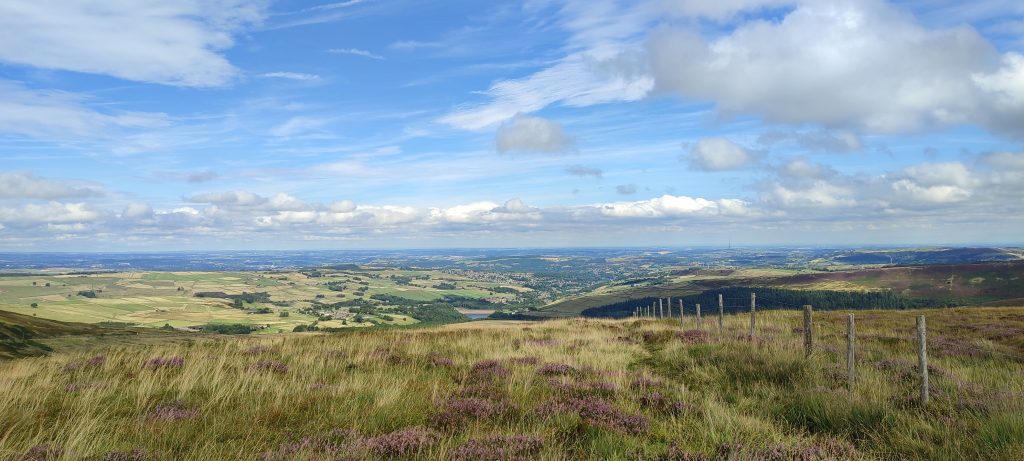
    How nature-rich corridors are to return to the banks of the River Holme between Holmfirth and Huddersfield

    A venture to develop ‘nature-rich’ corridors along nearly 22km of river and tributaries and revive endangered species along the River Holme in Huddersfield has been presented the eco-friendly mild by the Authorities.

    Nature’s Holme, led and managed by South Pennines Park, will be supported by cross sector partners such as River Holme Connections, Palladium, the College of Huddersfield, landowners and farmers. It covers an place of 2,800 hectares.

    South Pennines Park, situated between the Peak District, Yorkshire Dales, Increased Manchester, East Lancashire and West Yorkshire, is the premier non-statutory nationwide landscape in the Uk and dwelling to unusual birds such as merlin, limited-eared owl and twite.

    The scheme, based mostly in the south-east corner of South Pennines Park, will improve the River Holme – flowing from Holme village by means of cities which include Holmfirth, Honley and Meltham, to Huddersfield town centre.

    The pilot, one particular of 22 throughout the region to receive Federal government funding through the Landscape Restoration plan, and backed by the Section for Natural environment, Food and Rural Affairs (DEFRA) will involve groups of farmers and land supervisors operating collectively to deliver environmental advantages throughout farmed and rural landscapes – bettering soils, flood alleviation and water retention, increasing biodiversity carbon storage, and enhanced h2o excellent.

    With its large rainfall and neighborhood geology, South Pennines Park is a crucial place for h2o supply, with numerous reservoirs supplying h2o to nearby cities.

    The River Holme in all its glory. Pic by: SEAN DOYLE

    The two-year undertaking progress period of landscape restoration will start in winter season 2022-23, which will determine the scope of do the job and deliverables. This will be satisfied by a combination of community and personal financial commitment.

    Engagement with communities, farmers, landowners and crucial stakeholders will sort a vital portion of the approach – stimulating discussions, sharing information and forming designs.

    The venture will also be supported by a PhD scholar from the College of Huddersfield who will be assisting with measurement and analysis.

    Simon Hirst, river steward with River Holme Connections, which is supplying ‘boots on the ground’ help, stated: “The atmosphere has experienced traditionally thanks to industrialisation. The weirs and urbanisation of the river channel have intended the river has been closely modified.

    “There is an chance to make it extra normal by making biodiversity-prosperous corridors to benefit people today and wildlife.

    “We didn’t want to slim the scope of get the job done. Despite the fact that we had been successful with our bid for river and stream restoration, we can do a lot of do the job that will carry rewards to the watercourse – like planting and delivering patterns for wildlife.”

    The scheme will concentration on: fish migration centred on previous industrial weirs hedgerows and planting wildflower meadows peat restoration organic flood administration endangered species these kinds of as water voles and white-clawed crayfish the eradication of non-indigenous invasive crops such as Japanese knotweed and Himalayan balsam and sustainable funding.

    Helen Noble, chief government of South Pennines Park, reported: “The landscape restoration plan is currently being hailed by land professionals and conservationists as the most fascinating and vital step in a technology to restore misplaced biodiversity.

    “To halt the loss of habitats and species we have to have to act at a landscape scale, and pilots like Nature’s Holme are a important prospect to get this right and prove a scalable company model.

    “These initiatives will provide hectares of nature rich habitats, as perfectly as a sizeable selection of public items which includes carbon sequestration, reduced flood chance and biodiversity.

    “It is our goal that by 2038 the River Holme catchment will be resilient to local climate modify, a location in which mother nature and wildlife is connected and flourishing and communities, visitors, and company value, enjoy and care.”

    Property developer exploring mining possibilities at seaside beauty spot

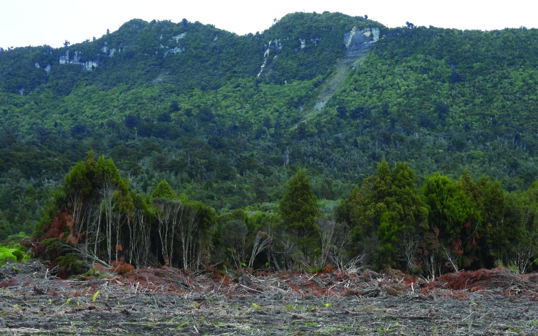
    The Rapahoe block, with work under way below the Twelve Apostles Range.

    The Rapahoe block, with function beneath way under the Twelve Apostles Selection.
    Photograph: Brendon McMahon / Greymouth Star

    A distinguished 16ha block bordering the seaside settlement of Rapahoe and State Highway 6 could be subdivided into way of life-measurement residential blocks.

    However, developer Terry Birchfield states he is also checking out the risk of mining the web site, which has a spectacular Twelve Apostles Selection backdrop.

    Tall flax and scrub and some bush re-growth has been flattened or cleared and new drains fashioned given that Birchfield acquired the assets previously this yr.

    Fox River resident Andrew Beaumont contacted the Greymouth Star involved that function might be destroying what appeared to be a normal wetland.

    “They are chopping into that regrowth of bush and placing in drains,” he mentioned. “It seems to me like a pretty massive indigenous wetland space that could be appeared following.”

    However, Birchfield stated the block was not naturally swampy, even with passing impressions. Run-off from the adjacent freeway intended water experienced nowhere else to go.

    “The street drain runs across into our location and there is no drain managing away from it, and it is really created a bloody mess of it. The road board (NZTA) is growling at me. We’re getting the water from the other side of the highway.”

    The internet site alone experienced great normal drainage on sand, about 1m to 1.5m beneath the prime layer of soil, he stated.

    The foreseeable future subdivision would be serviced with electricity and linked to drinking water, becoming near to services in Runanga and Rapahoe.

    Any progress was a pretty “gradual task” but the land was appealing for subdivision supplied its proximity to the coastline.

    At the very same time, test sampling for possible sand-primarily based mineral content experienced been carried out.

    “You will find all sorts of minerals close to these days. Gold is a person of them, but we’re all a bit ahead of our time,” Birchfield stated.

    West Coastline Regional Council acting consents and compliance supervisor Rachel Clark stated the council was aware of preliminary perform for some kind of potential progress along Rapahoe straight.

    “We are examining it, and we want to glimpse into it. I think they ended up undertaking most of what they were being undertaking less than permitted activity rules.”

    Gray District Council senior planner Michael McEnaney claimed the web site was not an discovered important normal location in the district prepare. Nor experienced it been discovered as an outstanding natural landscape or an spot of large normal character inside of the proposed Te Tai o Poutini Strategy.

    The NZ Transportation Company has been approached for comment.

    Local Democracy Reporting is Community desire journalism is funded by NZ on Air

    Binding affinity estimation from restrained umbrella sampling simulations

    Theoretical foundation

    Binding affinity is often quantified using the equilibrium dissociation constant (Kd), defined as:

    $$K_mathrmd = left[ mathrmP right]left[ mathrmL right]/left[ mathrmP:mathrmL right]$$

    (1)

    where [P], [L] and [P:L] are the concentrations of protein, ligand and the protein–ligand complex, respectively. Computationally, the absolute binding free energy (ΔG°), which is the standard molar free energy of binding, is more convenient to calculate. The dissociation constant and the absolute binding free energy are related via

    $$Delta G^circ = RTln fracK_mathrmd1,mathrmM$$

    (2)

    where R is the gas constant, T is the temperature and 1 M is 1 molar concentration. Various strategies have been used to estimate ΔG°, some of which were briefly discussed above. The methodology proposed here has a notable resemblance to the stratification strategy of refs. 3,4. However, the two methods have major differences as will be discussed later in this section.

    Absolute binding free energy or ΔG° is the free-energy change associated with moving the ligand from the bulk to the binding pocket (Supplementary Table 1). Within the formalism presented in this work, ΔG° is determined from the grid PMF G(x), where x is the position of the ligand mass center from the center of the binding pocket (Supplementary Table 1), G(x) is the PMF associated with the ligand position x. In practice, we need to bin the three-dimensional space and define the PMF at every bin or grid point as:

    $$Gleft( boldsymbolx right) = – RTln pleft( boldsymbolx right)$$

    (3)

    where p(x) is the probability of finding the ligand at bin x.

    We define ΔG(x) = G(x) − G(0), where x = 0 (that is, the center of the binding pocket) is defined as the grid point associated with the lowest grid PMF. One can show:

    $$Delta G^circ = – RTln frac{{int_mathrmpocket {mathrme^ – fracGleft( boldsymbolx right)RT} mathrmdV}}{{int_mathrmbulk {mathrme^{ – frac{Gleft( boldsymbolx right)}RT}} mathrmdV}} = – RTln frac{{int_mathrmpocket {mathrme^ – fracDelta Gleft( boldsymbolx right)RT} mathrmdV}}{{int_mathrmbulk {mathrme^ – fracDelta Gleft( boldsymbolx right)RT} mathrmdV}}$$

    (4)

    in which the binding ‘pocket’ refers to all x ∈ V where the ligand is considered bound and ‘bulk’ refers to all x ∈ V where the ligand is not interacting with the protein. V here is a subset of space with a single protein in standard concentration (that is, 1 M). As ΔG(x) is the same everywhere in the bulk, we can simplify relation (4) as follows:

    $$Delta G^circ = – RTln fracV_mathrmP{{mathrme^{ – frac{Delta Gleft( boldsymbolx_mathrmB right)}RT}V_mathrmB}} = – Delta Gleft( boldsymbolx_mathrmB right) – RTln fracV_mathrmPV_mathrmB$$

    (5)

    where VB is the bulk volume per protein associated with the standard concentration, xB is any grid point in the bulk and VP is the binding pocket volume defined as:

    $$V_mathrmP = mathop intnolimits_mathrmpocket {mathrme^{ – fracDelta Gleft( boldsymbolx right)RT}} mathrmdV$$

    (6)

    Defining ΔGV as the contribution of the difference between the volume of the binding pocket and the bulk to the binding free energy:

    $$Delta G_mathrmV = – RTln fracV_mathrmPV_mathrmB$$

    (7)

    Combining equations (5) and (7), we have:

    $$Delta G^circ = – Delta Gleft( boldsymbolx_mathrmB right) + Delta G_mathrmV$$

    (8)

    We can find the bulk volume (VB) associated with the standard concentration for a single protein approximately as:

    $$V_mathrmB = frac{frac1N_mathrmA,mathrmmol}{1,mathrmM} = frac1{N_mathrmA}mathrmL approx 1,661,mathrmAA^3$$

    (9)

    where NA is Avogadro’s constant and L is the unit of volume (litres). We can now rewrite ΔGV as:

    $$Delta G_mathrmV = – RTln fracV_mathrmPV_mathrmB = – RTln frac{V_mathrmP}mathrmAA^3 + RTln fracV_mathrmBmathrmAA^3 = Delta G_mathrmP – Delta G_mathrmB$$

    (10)

    in which ΔGB is the bulk volume contribution and ΔGP is the binding pocket contribution:

    $$left{ {beginarray*20l {Delta G_mathrmB = – RTln frac{{V_mathrmB}}{mathrmAA^3} approx – 7.42RT} hfill \ {Delta G_mathrmP = – RTln frac{{V_mathrmP}}{{mathrmAA^3}} = – RTln mathop intnolimits_mathrmpocket {mathrme^{ – frac{Delta Gleft( boldsymbolx right)}RT}} fracmathrmdV{{mathrmAA^3}}} hfill endarray} right.$$

    (11)

    Determining both ΔG(xB) and ΔGP requires finding the grid PMF ΔG(x). ΔG(xB) is the PMF difference between the binding pocket center and the bulk and ΔGP also requires an estimate for ΔG(x) within the binding pocket. We therefore do not need to find ΔG(x) for all x if we have a good estimate for ΔG(x) within the binding pocket and in the bulk. Ideally, ΔG(x) for these points can be determined by pulling the ligand out of the binding pocket towards the bulk and using an enhanced sampling technique such as US to sample the space of a collective variable such as d, that is, the distance between the mass centers of the ligand and protein. ΔG(x) can be estimated for all sampled grid points x using this distance-based US simulation. Note that the collective variable used for biasing would be d, while the collective variable used for the PMF calculations would be the three-dimensional position vector of the mass center of ligand with respect to protein’s binding pocket center. One may estimate the grid PMF from the distance-based US simulations using a non-parametric reweighting algorithm as discussed in this section. ΔG(x) can also be used to estimate ΔGP as defined in relation (11). There is often no need to strictly define the binding pocket as only low ΔG(x) values have non-negligible contribution to VP and thus even if we include all sampled grid points, only those close to the binding pocket center have non-negligible contributions.

    A practical issue with determining ΔG(xB) is the convergence. The key obstacles for the sampling that slow down the convergence are the orientation of the ligand, and the conformational changes of the ligand and protein. Using an approach similar in spirit to the previously proposed stratification strategy3,4,24, we can circumvent extensive sampling of these degrees of freedom. Let us first focus on the orientation of the ligand (Ω), defined using the orientation quaternion formalism. We can restrain Ω during the distance-based US simulations using a biasing potential ((frac12kvarOmega ^2) where a k is harmonic force constant) and later correct the free-energy difference based on the PMF associated with the Ω, which is different in the bulk (F(xB, Ω)) and in the binding pocket (F(0, Ω)). More generally, for any grid point x, we may determine ΔG(x) based on the PMF associated with the Ω at x (F(x, Ω)) and 0 (F(0, Ω)):

    $$mathrme^ – fracDelta G(boldsymbolx)RT = frac{{int_!0^uppi {mathrme^ – fracF(boldsymbolx,varOmega )RTmathrmdvarOmega } }}{{int_!0^uppi {mathrme^ – fracF(boldsymbol0,varOmega )RTmathrmdvarOmega } }}$$

    (12)

    Note that F(x, Ω) is the PMF associated with x and Ω, defined such that:

    $$Gmathrm(boldsymbolxmathrm) = c – RTln mathop intnolimits_!0^uppi {mathrme^{ – fracF(boldsymbolx,varOmega )RT}mathrmdvarOmega }$$

    (13)

    where c is an arbitrary constant. We therefore have:

    $$mathrme^{ – frac{Delta G(boldsymbolx)}RT} = frac{{int_!0^uppi {mathrme^{ – frac{F(boldsymbolx,varOmega )}RT}mathrmdvarOmega } }}{{int_!0^uppi {mathrme^ – fracF(boldsymbolx,varOmega ) + frac12kvarOmega ^2RTmathrmdvarOmega } }} times frac{{int_!0^uppi {e^ – fracF(boldsymbol0,varOmega ) + frac12kvarOmega ^2RTmathrmdvarOmega } }}{{int_!0^uppi {e^{ – fracF(boldsymbol0,varOmega )RT}mathrmdvarOmega } }} times frac{{int_!0^uppi {mathrme^{ – fracF(boldsymbolx,varOmega ) + frac12kvarOmega ^2RT}mathrmdvarOmega } }}{{int_!0^uppi {mathrme^{ – frac{F(boldsymbol0,varOmega ) + frac12kvarOmega ^2}RT}mathrmdvarOmega } }}$$

    (14)

    We now define GΩ(x) as the grid PMF of the restrained system (by Ω):

    $$G_varOmega (boldsymbolx) = – RTln mathop intnolimits_!0^uppi {mathrme^{ – frac{F(boldsymbolx,varOmega ) + frac12kvarOmega ^2}RT}mathrmdvarOmega }$$

    (15)

    We also define UΩ(x) as the average biasing potential at grid point x:

    $$U_varOmega left( boldsymbolx right) = – RTln langle mathrme^ – fracfrac12kvarOmega ^2RT rangle _boldsymbolx = – RTln frac{{int_0^uppi {mathrme^{ – frac{{Fleft( boldsymbolx,varOmega right) + frac12kvarOmega ^2}}RT}} mathrmdvarOmega }}{{int_0^uppi {e^{ – frac{{Fleft( boldsymbolx,varOmega right)}}RT}} mathrmdvarOmega }}$$

    (16)

    Now we have from relations (14), (15) and (16):

    $$Delta Gleft( boldsymbolx right) = Delta G_varOmega left( boldsymbolx right) – Delta U_varOmega left( boldsymbolx right)$$

    (17)

    where, the free energy of grid point x from the center 0 (ΔG(x)) is calculated based on its equivalent free energy (ΔGΩ(x)) in a system biased by a harmonic restraint on Ω and a correction term ΔUΩ(x). For x = xB:

    $$Delta U_varOmega left( boldsymbolx_mathrmB right) = – RTln frac{{langle mathrme^ – fracfrac12kvarOmega ^2RT rangle _mathrmbulk}}{{langle mathrme^ – fracfrac12kvarOmega ^2RT rangle _mathrmpocket}}$$

    (18)

    To determine the above ensemble averages, we need to determine the PMF along Ω for the bound and unbound ligand and calculate the ensemble averages analytically using relation (16). ΔGΩ(xB) can be determined from PMF calculations, where the distance between the protein and ligand is varied and the orientation of the ligand is restrained (distance-based BEUS with restrained orientation). We note that:

    $$V_mathrmP = mathop intnolimits_mathrmpocket {mathrme^{ – frac{{Delta Gleft( boldsymbolx right)}}RT}} mathrmdV = mathop intnolimits_mathrmpocket {mathrme^{ – frac{Delta G_varOmega left( boldsymbolx right) – Delta U_varOmega left( boldsymbolx right)}RT}} mathrmdV approx mathop intnolimits_mathrmpocket {mathrme^{ – frac{Delta G_varOmega left( boldsymbolx right)}RT}} mathrmdV$$

    (19)

    where we assume ΔUΩ(x) is negligible for x within the binding pocket. In other words, (langle {mathrme^ – fracfrac12kvarOmega ^2RT} rangle _boldsymbolx approx langle {mathrme^ – fracfrac12kvarOmega ^2RT} rangle _boldsymbol0) for x close to 0.

    In brief, if we choose to restrain the orientation, our absolute binding-free-energy estimate includes the following terms (using relations (8) and (17)):

    $$Delta G^circ = – Delta G_varOmega left( boldsymbolx_mathrmB right) + Delta U_varOmega left( {boldsymbolx_mathrmB} right) + Delta G_mathrmV$$

    (20)

    F(xB, Ω) can be calculated numerically from orientation angle distribution of a free ligand: (F(boldsymbolx_mathrmB,varOmega ) = – RTln pleft( varOmega right),) where p(Ω) is determined from the distribution of Euler angles ((pleft( phi ,theta ,psi right) = frac18uppi ^2sin theta), where 0 ≤ ϕ, ψ ≤ 2π and 0 ≤ θ ≤ π) given that:

    $$cos fracvarOmega 2 = cos fracphi 2cos fractheta 2cos fracpsi 2 + sin fracphi 2sin fractheta 2sin fracpsi 2$$

    (21)

    (langle {mathrme^ – fracfrac12kvarOmega ^2RT} rangle _{mathrmbulk}) can then be calculated using relation (16) with numerically estimated F(xB, Ω) and the k value used in the simulations. (Fleft( {boldsymbolx_mathrmB,varOmega } right) = – RTln p(varOmega )) was numerically estimated by discretizing each of the 3 Euler angles with a bin width of 1° and a total of 360 × 360 × 180 bins to estimate p(Ω) from p(ϕ, θ, ψ). F(0, Ω) can be determined approximately using orientation-based US simulations of bound ligand. F(0, Ω) can then be used to estimate (langle {mathrme^{ – fracfrac12kvarOmega ^2RT}} rangle _mathrmpocket) using relation (16).

    The above strategy can be extended to other degrees of freedom for which unbiased sampling may hinder the convergence. Most notably, the internal conformational changes of the ligand and that of the protein may also play a crucial role in slowing down the convergence. In the following, we show how one can restrain not only the orientation of the ligand but also the RMSD of the ligand (denoted here by r) in distance-based US simulations (along d) to speed up convergence. In this case, the grid PMF difference ΔG(x) is calculated based on ΔGΩ,r(x), the grid PMF of a system whose Ω and r are both restrained:

    $$mathrme^{ – frac{{Delta Gleft( boldsymbolx right)}}RT} = frac{{int_!0^infty {int_0^uppi {mathrme^{ – frac{{Fleft( {boldsymbolx,varOmega ,r} right)}}RT}} } mathrmdvarOmega mathrmdr}}{{int_!0^infty {int_!0^uppi {mathrme^{ – fracFleft( boldsymbol0,varOmega ,r right)RT}} } mathrmdvarOmega mathrmdr}}$$

    (22)

    Using a similar strategy as in relation (14), we have:

    $$beginarraylmathrme^ – fracDelta Gleft( x right)RT = frac{{mathop smallint nolimits_0^infty mathop smallint nolimits_0^uppi mathrme^{ – frac{{Fleft( {boldsymbolx,Omega ,r} right)}}RT}mathrmdvarOmega mathrmdr}}{{mathop smallint nolimits_0^infty mathop smallint nolimits_0^uppi mathrme^{ – frac{{Fleft( {boldsymbolx,varOmega ,r} right) + frac12k^prime r^2}}RT}mathrmdvarOmega mathrmdr}} times frac{{mathop smallint nolimits_0^infty mathop smallint nolimits_0^uppi mathrme^{ – frac{{Fleft( {boldsymbolx,varOmega ,r} right) + frac12k^prime r^2}}RT}mathrmdvarOmega mathrmdr}}{{mathop smallint nolimits_0^infty mathop smallint nolimits_0^uppi mathrme^{ – frac{{Fleft( {boldsymbolx,varOmega ,r} right) + frac12k^prime r^2 + frac12kvarOmega ^2}}RT}mathrmdvarOmega mathrmdr}}\ times frac{{mathop smallint nolimits_0^infty mathop smallint nolimits_0^uppi mathrme^ – fracFleft( 0,varOmega ,r right) + frac12k^prime r^2 + frac12kvarOmega ^2RTmathrmdvarOmega mathrmdr}}{{mathop smallint nolimits_0^infty mathop smallint nolimits_0^uppi mathrme^{ – fracFleft( boldsymbol0,varOmega ,r right) + frac12k^prime r^2RT}mathrmdvarOmega mathrmdr}} times frac{{mathop smallint nolimits_0^infty mathop smallint nolimits_0^uppi mathrme^{ – frac{{Fleft( boldsymbol0,varOmega ,r right) + frac12k^prime r^2}}RT}mathrmdvarOmega mathrmdr}}{{mathop smallint nolimits_0^infty mathop smallint nolimits_0^uppi mathrme^{ – frac{{Fleft( boldsymbol0,varOmega ,r right)}}RT}mathrmdvarOmega mathrmdr}}\ times frac{{mathop smallint nolimits_0^infty mathop smallint nolimits_0^uppi mathrme^{ – frac{{Fleft( {boldsymbolx,varOmega ,r} right) + frac12k^prime r^2 + frac12kvarOmega ^2}}RT}mathrmdvarOmega mathrmdr}}{{mathop smallint nolimits_0^infty mathop smallint nolimits_0^uppi mathrme^{ – frac{Fleft( boldsymbol0,varOmega ,r right) + frac12k^prime r^2 + frac12kvarOmega ^2}RT}mathrmdvarOmega mathrmdr}}endarray$$

    (23)

    which results in:

    $${rme^{ – fracDelta Gleft( bfx right)RT}} = frac{{{{langle {rme^ – fracfrac12k^prime r^2RT}rangle }_bf0}}}{{{{langle {rme^{ – fracfrac12k^prime r^2RT}}rangle }_bfx}}} times frac{{{{langle {rme^{ – fracfrac12kvarOmega ^2RT}}rangle }_}0^r}}{{langle {rme^{ – frac{{frac12kvarOmega ^2}}RT}}rangle _bfx^r}} times frac{{rme^ – beta G_varOmega ,r(bfx)}}{{rme^ – beta G_varOmega ,r(bf0)}}$$

    (24)

    Here we have defined GΩ,r(x) as:

    $$G_varOmega ,rleft( boldsymbolx right) = – RTln mathop intnolimits_0^infty {mathop intnolimits_0^uppi {mathrme^{ – frac{{Fleft( {boldsymbolx,varOmega ,r} right) + frac12k^prime r^2 + frac12kvarOmega ^2}}RT}} }$$

    (25)

    where k′ is the harmonic force constant associated with the r based on biasing potential ((frac12k^prime r^2)). We also define Ur(x) similar to UΩ(x) in relation (15) except for using r instead of Ω. (U_varOmega^r(boldsymbolx)) is also defined similar to UΩ(x) except for the additional restraint on r:

    $$U_varOmega ^rleft( x right) = – RTln langle {mathrme^{ – frac{{frac12kvarOmega ^2}}RT}} rangle _boldsymbolx^r = – RTln frac{{mathop smallint nolimits_0^infty mathop smallint nolimits_0^uppi mathrme^{ – frac{{Fleft( {boldsymbolx,varOmega ,r} right) + frac12k^prime r^2 + frac12kvarOmega ^2}}RT}mathrmdvarOmega mathrmdr}}{{mathop smallint nolimits_0^infty mathop smallint nolimits_0^uppi mathrme^{ – frac{{left( {Fleft( {boldsymbolx,varOmega ,r} right) + frac12k^prime r^2} right)}}RT}mathrmdvarOmega mathrmdr}}$$

    (26)

    Finally, we have:

    $$Delta Gleft( boldsymbolx right) = Delta G_{varOmega ,r}left( {boldsymbolx} right) – Delta U_rleft( {{{boldsymbolx}}} right) – Delta U_{varOmega }^rleft( {{{boldsymbolx}}} right)$$

    (27)

    In brief, if we choose to restrain both the orientation and RMSD, our absolute binding-free-energy estimate includes the following terms:

    $$Delta G^circ = – Delta G_varOmega ,rleft( {{{{boldsymbolx}}}_mathrmB} right) + Delta U_rleft( {{{{boldsymbolx}}}_mathrmB} right) + Delta U_varOmega ^rleft( {{{{boldsymbolx}}}_mathrmB} right) + Delta G_mathrmV$$

    (28)

    Here we are using an approximation similar to that in relation (19):

    $$V_mathrmP approx mathop intnolimits_mathrmpocket {mathrme^{ – frac{{{{Delta }}G_{{{varOmega }},r}left( {{{boldsymbolx}}} right)}}{RT}}} mathrmdV$$

    (29)

    Using relations (20) and (28), we can generalize the stratification strategy to include three restraints on arbitrary collective variables α, β and γ:

    $$Delta G^circ = – Delta G_alpha ,beta ,gamma left( {{{{boldsymbolx}}}_mathrmB} right) + Delta U_gamma left( {{{{boldsymbolx}}}_mathrmB} right) + Delta U_beta ^gamma left( {{{{boldsymbolx}}}_mathrmB} right) + Delta U_alpha ^beta ,gamma left( {{{{boldsymbolx}}}_mathrmB} right) + Delta G_mathrmV$$

    (30)

    where:

    $$Delta G_mathrmV approx – RTln mathop intnolimits_{{mathrmpocket}} {mathrme^{ – frac{{Delta G_alpha ,beta ,gamma ({{{boldsymbolx}}})}}{{RT}}}} frac{mathrmdV}{{{mathrmAA}^3}} – Delta G_mathrmB$$

    (31)

    Isothermal titration calorimetry of hFGF1 with heparin hexasaccharide

    ITC data were obtained using MicroCal iTC 200 (Malvern) with microcal origin software. The change in heat during the biomolecular interaction was measured by titrating heparin (loaded in the syringe) into the hFGF1 solution in the calorimetric cell. Both the protein and the heparin samples were prepared in the buffer containing 10 mM phosphate buffer with 100 mM NaCl at pH 7.2 and were degassed before loading. The protein-to-heparin ratio was maintained at 1:10 with the protein concentration being 100 μM and the heparin concentration being 1 mM. A total of 30 injections were conducted with a constant temperature of 25 °C and stirring speed of 300 rpm. One set of sites binding model was used for the ITC binding curve68. The standard binding free energy ΔG° was determined from dissociation constant via relation (2) at T = 25 °C. The experiment was repeated three times with the same sample and the results obtained were very similar to each other. The mean and standard deviation were reported for both Kd and ΔG°.

    All-atom MD simulations

    For our bound state, we utilized the X-ray crystal structure of the dimeric hFGF1 combination with heparin hexasaccharide (PDB 2AXM; resolution, 3.0 Å)69, and for our apo state, we used the X-ray crystal structure of monomeric hFGF1 (PDB 1RG8; resolution, 1.1 Å)70. The NAMD 2.13 (ref. 71) was used to run MD simulations. Using a conjugate gradient, we energy-minimized the system for 10,000 steps. We next relaxed the systems using stepwise restrained MD simulations (for 1 ns) using CHARMM-GUI72. All production runs were done in an NPT (constant N, number of atoms; P, pressure; T, temperature) ensemble after the first NVT (constant N, number of atoms; V, volume; T, temperature) relaxation. Simulations were done at 300 K with a 2 fs time step and a 0.5 ps−1 damping coefficient using a Langevin integrator. Nosé–Hoover–Langevin pistons were used to maintain 1 atm pressure72. Long-range electrostatic interactions were estimated using the particle mesh Ewald approach. The initial runs were done for 15 ns, followed by the production run on the Anton 2 supercomputer (Pittsburgh Supercomputing Center) for 4.8 μs with a 2.5 fs time step.

    MD simulations of free heparin hexasaccharide

    Heparin hexasaccharide69 was simulated in a rectangular water box without the protein. The system was set up as described previously in the ‘All-atom MD simulations’ section. The final conformation after relaxation was then used as the starting conformation for 10 production runs for 40 ns each. The total simulation time was around 400 ns.

    SMD simulations

    The final conformations of the hFGF1–heparin73, apo hFGF1 (ref. 73) and free heparin hexasaccharide equilibrium simulations were used to generate starting conformations for the non-equilibrium pulling simulations. Four collective variables74 were used for the SMD simulations75: (1) distance between the heavy-atom center of mass of heparin and that of the protein (d); (2) the orientation angle of heparin with respect to the protein (Ω) defined using the orientation quanternion formalism; (3) RMSD of the protein (rP); (4) RMSD of heparin (rL). Six independent sets of simulations were performed. The distance-based SMD simulation was run for 9.5 ns, while the orientation-based SMD simulation was run for 8 ns. The distance-based SMD simulation was used to pull the heparin away from the protein by approximately 30 Å (10 Å → 40 Å) with a force constant of 100 kcal (mol Å2)−1. The orientation angle was also restrained in this simulation with a force constant of 0.5 kcal (mol degree2)−1 to stay close to its initial orientation in the bound state. The orientation-based SMD simulation was used to rotate the bound heparin locally with respect to the protein (0° → 73°) with a force constant of 100 kcal (mol degree2)−1. Four RMSD-based SMD simulations were run for 10 ns each using a force constant of 50 kcal (mol Å2)−1: (1) to change the RMSD of the bound protein (0.5 Å→2 Å) (the RMSD of heparin was restrained in this simulation with a force constant of 1 kcal (mol Å2)−1); (2) to change the RMSD of the bound heparin (1.5 Å → 4 Å); (3) to change the RMSD of the unbound protein (0.8 Å → 3.2 Å); (4) to change the RMSD of the free heparin (1.5 Å → 5.5 Å).

    BEUS simulations

    BEUS53,76,77, which is a variation of the US simulation method, was performed to estimate grid PMF (Supplementary Fig. 1). Four independent sets of distance (d)-based BEUS simulations were performed, with no restraints, restraint on orientation angle of heparin with respect to the protein (Ω), restraint on RMSD of the ligand (rL) and RMSD of the protein (rP), and restraints on Ω, rL and rP. Two sets of BEUS simulations were also performed using the Ω collective variable, one with and one without a restraint on rL and rP. In addition, two sets of BEUS simulations were performed using the rP collective variable (bound protein with restraint on rL; unbound protein) and two sets were performed using the rL collective variable (bound ligand; free ligand). Selected SMD conformations were assigned to individual BEUS windows with equal spacing in each one of these BEUS simulations. The distance-based BEUS simulations ran for 10 ns with 31 replicas/windows and the orientation-based simulations ran for 10 ns with 30 replicas/windows. The RMSD-based BEUS simulations ran for 10 ns with 12 replicas/windows. The force constant used for ligand–protein distance (d) in distance-based BEUS was 2 kcal (mol Å2)−1 while the orientation was restrained as in SMD simulations using a force constant of 0.5 kcal (mol degree2)−1. For orientation-based BEUS simulations, the force constant for the ligand orientation angle (as in SMD simulations) was set to 0.5 kcal (mol degree2)−1. The force constant used for rL and rP in all cases was 1 kcal (mol Å2)−1. See Supplementary Fig. 1 for a schematic representation of these simulations.

    Free-energy calculations using non-parametric reweighting

    Once the BEUS simulations described above were converged, a non-parametric reweighting method76,78, which is somewhat similar to the multi-state Bennett acceptance ratio method79, was used to construct the PMF. In this method76, each sampled configuration will be assigned a weight, which can be used to construct the PMF in terms of a desired collective variable. Suppose that a system is biased (for instance, within a BEUS scheme) using N different biasing potentials Ui(r), where i = 1, …, N, and r represents all atomic coordinates. Typically, Ui(r) is a harmonic potential defined in terms of a collective variable with varying centers for different i. Assuming an equal number of sampled configurations from each of the N generated trajectories, we can combine them in a single set of samples rk (irrespective of which bias was used to generate each sample rk) and determine the weight of each sample (wk) as:

    $$w_k = c/mathop sumlimits_i {mathrme^{ – frac{{left( {U_ileft( boldsymbolr_k right) – F_i} right)}}{{RT}}}}$$

    (32)

    where, c is the normalization constant such that (mathop sumnolimits_k w_k = 1) and both wk and perturbed free energies Fi are determined iteratively using the above equation and the following:

    $$mathrme^ – beta F_i = mathop sumlimits_k {w_kmathrme^{ – frac{{U_ileft( boldsymbolr_k right)}}{{RT}}}}$$

    (33)

    Converged wk values can be used to construct any ensemble averages including any PMF (for example, G(ζ) PMF of the atomic system in the collective variable space(ζ))) in terms of not only the collective variable used for biasing but also any other collective variables that are sufficiently sampled. One may use a weighted histogram method to construct the PMF as follows:

    $$Gleft( boldsymbolupzeta _i right) = – RTln mathop sumlimits_k w_k delta left( {boldsymbolupzeta left( {boldsymbolr_k} right) – boldsymbolupzeta _i} right),$$

    (34)

    $$delta left( {boldsymbolupzeta left( {{{boldsymbolr}}_k} right) – boldsymbolupzeta _i} right) = left{ {beginarray*20l 1, hfill & {left| {boldsymbolupzeta left( {{{{boldsymbolr}}}_k} right) – {{boldsymbolupzeta }}_i} right| < left| {{{{boldsymbolupzeta }}}left( {{{{boldsymbolr}}}_k} right) – {{{boldsymbolupzeta }}}_j} right|mathrmfor,j ne i.} hfill \ 0, hfill & mathrmotherwise hfill endarray} right.$$

    (35)

    To estimate the uncertainty of any of PMF calculations described above, one may use bootstrapping. Here, we have used a block Bayesian bootstrapping technique77, where 100 alternative datasets are resampled from the existing dataset and the same non-parametric reweighting algorithm and the same PMF calculation is repeated for each set to generate 100 alternative PMFs. The standard deviation of the PMF at any point along the reaction coordinate provides an estimate for the error.

    Alchemical FEP simulations

    We used the BFEE2 (ref. 27) package to estimate the absolute free energy of binding in silico for an alchemical or geometrical route with multiple subprocesses and geometric constraints. Alchemical FEP simulations were performed to calculate the absolute binding free energy for the interaction of hFGF1 with heparin hexasaccharide. We used a double annihilation protocol80, wherein the heparin hexasaccharide is annihilated in both the free and bound states. The final conformations of the hFGF1–heparin complex73 and free heparin hexasaccharide equilibrium simulations (discussed previously in the ‘All-atom MD simulations’ section) were used to generate starting conformations for the bound hFGF1–heparin and free heparin FEP simulations respectively. For the alchemical route, four separate simulations are performed: (1) coupling the restraints of seven collective variables in the bound state; (2) decoupling the ligand alchemically in the bound state; (3) coupling the ligand alchemically in the unbound state; (4) decoupling the conformational restraints in the unbound state. The FEP simulations 1 and 3 were performed bidirectionally using 200 λ-windows (λ is the coupling parameter associated with the FEP that could vary between 0 and 1). Each λ-window included a 0.5 ns of equilibration and 5.0 ns of averaging for both the unbound and bound states, for a total of 2.3 μs (Supplementary Table 3). The decoupling FEP simulations 2 and 4 were also performed bidirectionally, each one for 51 ns. All FEP simulations were performed using the NAMD 2.13 (ref. 71) simulation package with the CHARMM36m all-atom additive force field, using the protocol discussed previously for the equilibrium simulations. We used the state-of-the-art BFEE2 (ref. 27) method to make input files and analyze the FEP simulations.

    Binding-free-energy calculations using geometrical route

    The extended ABF technique with an umbrella integration estimator was used to calculate the free-energy change along the coarse variables required to characterize reversible heparin–hFGF1 binding3,24,27. We used the software BFEE2 (ref. 27) to generate the input files for these simulations. In the geometrical route, these collective variables are often subjected to restrictions, and the amount of reversible work required to impose each constraint is determined by a sequence of very accurate PMF simulations. The collective variables used here are the RMSDs of the two proteins’ backbone distances from the reference, native conformation, the three Euler angles (Θ, Φ and Ψ) that describe their relative orientation and the polar (θ) and azimuth angles (φ) that describe their relative position27,81. The geometrical path consists of a sequence of separate PMF computations performed sequentially with the gradual inclusion of restrictions (RMSD, Θ, Φ, Ψ, θ and φ), as shown in Supplementary Table 2. Each geometric collective variable (RMSD, Θ, Φ, Ψ, θ, φ and r = (1/β) ln(S*I*C°); β = (𝑘BT)−1, with kB the Boltzmann constant and T the temperature; C° denotes the standard concentration of 1 M. I*, which stands for the separation term, and S*, which stands for the surface term, indicate the percentage of a sphere with radius r*, centered at the binding site of the reference protein, that is, accessible to its partner) simulation was run with 10 replicas per restriction, and each replica simulation included 20 ns (RMSD, Θ, Φ, Ψ, θ and φ) of simulation time (r collective variables simulations were run for 40 ns for each replica), for a total of 1.6 μs. The BFEE2 (ref. 27) Gui was used to analyze the final ABF simulation data.

    Reporting summary

    Further information on research design is available in the Nature Portfolio Reporting Summary linked to this article.